Abstract
Prior to every geostatistical estimation or simulation study there is a need for de-limiting the geologic domains of the deposit, which is traditionally done manually by a geomodeler in a laborious, time consuming and subjective process. For this reason, novel techniques referred to as implicit modelling have appeared. These techniques provide algorithms that replace the manual digitization process of the traditional methods by some form of automatic procedure. This paper covers a few well estab-lished implicit methods currently available with special attention to the signed distance function methodology. A case study based on a real dataset was performed and its applicability discussed. Although it did not replace an experienced geomodeler, the method proved to be capable in creating semi-automatic geological models from the sampling data, especially in the early stages of exploration.
Keywords: implicit geologic modeling, signed distance function, domaining.
Roberto Mentzingen Rolo
Mestrando
Universidade Federal do Rio Grande do Sul - UFRS Departamento de Engenharia de Minas Porto Alegre – Rio Grande do Sul – Brasil [email protected]
Ricardo Radtke
Mestrando
Universidade Federal do Rio Grande do Sul - UFRS Departamento de Engenharia de Minas Porto Alegre – Rio Grande do Sul – Brasil [email protected]
João Felipe Coimbra Leite Costa
Professor titular
Universidade Federal do Rio Grande do Sul - UFRS Departamento de Engenharia de Minas Porto Alegre – Rio Grande do Sul – Brasil [email protected]
Signed distance function
implicit geologic modeling
Mining
Mineração
http://dx.doi.org/10.1590/0370-44672016700146
1. Introduction
The necessary investment to start a mine is in the order of tens to hundreds of millions of dollars. For the investment to be proitable, the potential product in the subsurface must be present in adequate quantity and quality to justify a decision to invest.
All technological and inancial de-cisions are built on the knowledge about the mineral deposit. Thus, the estimation of grade and location of material in the ground (in situ resources) must be known with an acceptable degree of conidence. A small difference between planned (es-timated) and realized production have a large impact on mine profitability (Sinclair and Blackwell, 2002).
The resource evaluation of a min-ing deposit is composed of two steps (Chilès et al., 2004): Delimitation of the boundaries of the units correspond-ing to the various geological formations and estimation or simulation of grades within each unit.
Therefore, prior to every geosta-tistical estimation or simulation, there is a need for delimiting the geologic
for geological and statistical homogene-ity within chosen domains (McLennan, 2007). Generating accurate boundary models is clearly necessary, as the qual-ity of the models will inluence various downstream mine practices, including estimations/simulations and mining planning (Cowan et al., 2003). These boundaries, separating different station-ary domains, are traditionally modeled explicitly by manual digitizing from sample data.
First, two-dimensional poly-lines are manually drawn on cross sections honoring the sample data, and then linked by tie lines, these tied poly-lines are triangulated to create a wire-frame that represents a geologic unit, this process has some disadvantages (Cowan et al., 2003): its time consuming and requires an experienced geomodeler to construct complex geometries; the model produced is unique to each in-dividual geomodeler, and cannot be replicated, making auditing by external personnel a hard task; it is inlexible, since modifying the model as new data
and laborious.
For most mines, only a single work-ing model is maintained because of the time constraint. Rarely is there an oppor-tunity to model alternative interpreta-tions and compare resource estimainterpreta-tions based on the alternative models; thus, the assessment of mining risks is avoided, even though it is inherent in geological modeling (Cowan et al., 2003).
Mining software packages have provided computational tools to dis-play drillhole data and to speed up the manual digitization of cross sections. Despite these advances, explicit model-ing still suffers from the disadvantages presented. Recent novel techniques referred to as implicit modeling provide algorithms that reduce the level of sub-jectivity by replacing the digitization process with some form of automatic procedure (Silva, 2015).
2. Geologic modeling
There are two groups of geologic modeling techniques available:
1) Deterministic techniques, which comprise explicit methods where the boundary that separates the geological domains is defined explicitly by the geomodeler, in vertical and horizontal sections, from the drillhole data and implicit methods which replace the manual digitization of the explicit meth-ods by an automatic or semi-automatic
form of domain delimitation. Implicit methods are straightforward and com-putationally fast. Some well-established implicit methodologies are reviewed in this paper: The Leapfrog© methodology
(Cowan et al., 2003), potential ield (Chilès et al., 2004) and signed distance function technique (Deutsch and Wilde, 2013; Silva, 2015). For the latter, a special plug-in was developed to run at SGeMS. A real case study is presented
herein to illustrate the methodology. 2) Stochastic techniques require more computational effort, and are not so straightforward. The established algorithms are: sequential indicator simulation (Journel, 1989b), trun-cated gaussian simulation (Journel and Isaaks, 1984), plurigaussian simulation (Galli et al., 1994) and multi-point based methods (Guardiano and Sriv-astava, 1993).
3. Implicit methods
3.1
Leapfrog
©methodology
The subject was introduced in the geology ield by Cowan et al., (2003), based on the work of Savchenko et al., (1995) for modeling objects interpolat-ing volume functions. The deinition of a volume function is attached to the no-tion of distance to an interface where the interface is deined as the surface sepa-rating two distinct domains. Distance is measured to the nearest interface, and it can be negative or positive depending on whether the location is inside or outside of the domain. The bounding interface of interest is the surface corresponding to a particular iso-value of the volume function, usually the iso-surface zero
(McLennan, 2007). The volume func-tion must be interpolated in order to deine the boundary interface, by imple-menting a fast scattered interpolator method know as radial basis function (RBF) (Hardy, 1990). The interpolator is represented as the linear combination of basic functions similar to dual kriging (Journel, 1989a).
Leapfrog© provides one of the irst
implicit boundary modeling implemen-tations within a commercial software package. There are ive major steps in the methodology (McLennan, 2007): (1) data validation and composting; (2) interpolation and meshing; (3)
incor-porating geological morphology; (4) interpolating the geological morphol-ogy; (5) morphologically constrained interpolation.
RBF functions do not derive the covariance functions from the data; they correspond to a simple isotropic linear covariance function. Therefore, there is no possibility of incorporating anisotropy into the boundaries through RBF interpolation. Instead it is injected manually in the form of deterministic morphological constraints (McLen-nan and Deutsch, 2006). Besides this, dealing with multiple domains is not straightforward (McLennan, 2007).
3.2 Potential field
Presented by Chiles et al., (2004), this is an implicit 3D scalar ield from which a geological interface is extract-ed as a particular iso-surface. There are ive major steps to the methodology (McLennan and Deutsch, 2006): (1) collect surface intersection and struc-tural orientation data; (2) determine
the form of the locally varying drift; (3) infer the potential ield covariance function; (4) interpolate the potential ield with the universal cokriging ap-proach; (5) visualize the uncertainty in the boundary surface placement.
A key feature of the potential ield method is the use of universal
cokriging to optimally account for both intersection and structural dip data. The procedure is not sim-ple, the covariance of the potential ield is particularly dificult to infer, since there are no hard potential ield data available (McLennan and Deutsch, 2006).
3.3 Distance function modeling
Signed distance function meth-odology for multiple categories (Silva, 2015) is a deterministic implicit model-ing technique where the implicit func-tion is constructed by interpolating a distance measure based on conditioning data. This method is based on the vol-ume function technique, however, someinteresting modifications were made (Silva, 2015).
For each sample, an anisotropic (or isotropic) distance between itself and the nearest sample belonging to an opposite domain is computed and assigned. Nega-tive values represent the distance to the boundary for samples inside the domain.
The interface that separates the regions in space is determined by the sign of the estimated signed distance values. The algorithm works as follows.
The set of data z(uα),α = 1,...,n
is coded in indicators to specify the samples that belong inside or outside of the domains (Equation 1).
=
outside
is
u
z
if
inside
is
u
z
if
u
i
)
(
,
0
)
(
,
1
)
(
(1)algorithm was applied in a real gold de-posit, results discussed and the implicit
compared to an explicit model created by a geomodeler, in order to check if
A simple two-dimensional example (Figure 1) proposed by Silva (2015) is presented to illustrate the process.
Figure 1
Simple two dimensional example illustra-ting Signed distance function modeling workflow, adapted from Silva (2015).
Signed distance values are then calcu-lated for each sample using Equation 2. If
the sample is inside the domain, the distance is negative; if the sample is outside the
do-main, the distance is positive. The euclidean norm is used to measure the distance.
=
+
=
=
0
)
(
,
||
||
1
)
(
,
||
||
)
(
u
i
if
u
u
u
i
if
u
u
u
d
(2) (3) (4)The location uβ corresponds to the
closest sample of the opposite domain to uα.
The distances can also be anisotro-pic, in this case, the set of data coordinates
x, y and z must be rotated and dilated (or
contracted), using the Equation 3 trans-formation, to x'', y'', z'', and then, the
eu-clidean distances are calculated normally.
Anisotropic distances should be used when it is known that the geologic body extends more in a speciic direction than in the oth-ers, as in the case of a tabular body.
= z y x z y x vert a a a cos cos cos sin cos sin sin cos sin sin sin cos sin cos cos cos sin sin cos sin sin cos cos sin sin sin sin cos cos 0 0 0 0 0 0 '' '' '' 1 1 1 min max
Where α, β and φ are azimuth, dip and rake respectively, and amax, amin and avert are the anisotropy ranges.
The signed distance implicit
func-tion is then interpolated to all locafunc-tions of interest (Equation 4). Ordinary krig-ing will be used due to its ability to ac-count for directions of continuity and
the spatial coniguration of data. Others techniques, such as inverse distance can also be used.
=
=
n
OK
u
d
u
u
d
1)
(
)
(
)
(
*
Deutsch and Wilde, (2013) rec-ommend the use of global kriging (Neufeld and Wilde, 2005), a smooth interpolator, to avoid artifacts in the implicit model. However the use of global kriging is restricted to the num-ber of samples due to computational eficiency. Instead of global kriging, ordinary kriging can be used consider-ing a large neighborhood and a large amount of data. Kriging allows us to control the run-time by changing the number of samples retained in the es-timates, while methods based on RBF
always use all samples.
The signed distances have a non-stationary behavior, namely, the var-iograms do not have a sill. Also, the linearity of the distance makes the origin behave close to a quadratic form. Thus, the Gaussian model is a well-suited structure for modeling this type of variogram. Known geological trends can be incorporated into the model by the variogram, whilst RBF based methods are not able to incor-porate anisotropy. An increment in the nugget effect disconnects the domains
and variations in the range inluence the shape and spatial extension of the geologic domains.
At the end, the domains are classi-ied at the unsampled location u in
func-tion of the sign of the signed distance estimates (Equation 5). If the estimate is negative, the location is classiied as inside the boundary; otherwise, the lo-cation is considered as outside. Models can be created in any resolution at the cost of computer resources and time, the resolution is controlled by modify-ing the dimensions of the grid blocks.
3.3.1 Distance function modeling for multiple geologic domains
The described signed distanceimplicit geologic modeling methodol-ogy may only be applied for binary cases. In that which follows, the
al-gorithm developed by Silva (2015) to handle multiple domains will be presented.
Suppose there exists K multiple
domains in the deposit. For all sample locations z(uα),α = 1,...,n, an indicator
vector of K elements is coded according
to Equation 6:
=
=
=
k
K
otherwise
u
z
if
k
u
z
if
u
i
k1
,...,
)
(
,
0
)
(
,
1
)
(
(6) (7)Thus the k element of the vector is
one while the remainder K-1 elements are
set to code 0.
In the same manner as in Equation 6, the signed distance value to the closest opposite domain is computed individually
for each k element of the vector (Equation 7). The signs of the distances remain equal as in the binary case.
K
k
u
i
if
u
u
u
i
if
u
u
u
d
k kk
1
,...,
0
)
(
,
||
||
1
)
(
,
||
||
)
(
=
=
+
=
=
Interpolation is performed individually for each k. Ordinary kriging is applied multiple times (Equation 8).
=
=
=
n k OKk
u
u
d
u
k
K
d
1 *,...,
1
)
(
)
(
)
(
(8)Then the inal rock type model is determined by the following equation.
{
}
Kk k
k
d
u
d
that
such
k
u
i
* * 1'
min
(
)
'
)
(
*
=
=
= (9)The estimated distance provides a measure of proximity to the closest
oppo-site domain. In this sense, the minimum es-timated signed distance value may be seen
as the most probable domain to be found at an unsampled location (Silva, 2015).
3.3.2 Measure of uncertainty (softmax transformation)
The proposed algorithm doesnot characterize uncertainty. There-fore, a heuristic measure of uncer-tainty was proposed by Silva (2015), this measure of uncertainty is not based on multiple realizations drawn
from a random function as in sto-chastic methods; Instead, it is based on a post-processing transformation method, a widely used approach for multiple class classiication (McCul-lagh and Nelder, 1989).
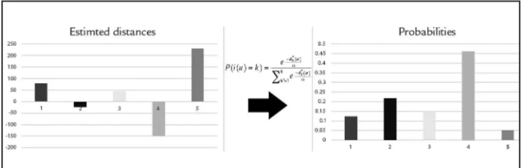
The central idea is to transform the estimated signed distance into values that can be interpreted as posterior probabilities (Equation 10). The transformed values lie between 0 and 1 and sum to 1 for all elements k .
=
=
=
k k u d u d k ke
e
k
u
i
P
1 ' ) ( ) ( * *)
)
(
(
(10)P(i(u))=k represents the
probabil-ity at location u to belong to category
k, d*
k (u) is the estimated distance for
category k and ω is a parameter that controls the uncertainty bandwidth for
K categories, a large parameter leads to
greater uncertainties.
To illustrate how the transforma-tion works Figure 2 shows, on the left, estimated distances for ive different
rock types on a particular block and on the right, the probabilities of this block to belong to each of the ive categories obtained from the distances by the softmax transformation.
Figure 2 Estimated distances and probabilities
obtained by softmax transformation for five rock types on a particular block.
The shorter the estimated distance for a given category K at an unknown
location u, the greater is the probability
3.3.3 Reproducing target proportions (servo system)
To avoid bias introduced bypref-erential sampling in geologic models, Silva (2015) proposed the use of some sample declustering techniques and the application of a servo system (Strebelle, 2002), to generate geologic models that
match the representative proportions on the declustered data.
The algorithm is based on the probabilities obtained after the distance transformation (Equation 10). The core of the algorithm (Equation 11) consists
of updating the probabilities of the do-mains based on the difference between the target and current marginal distribu-tions. The nodes visited must follow a random path to avoid the introduction of artifacts.
(11)
(12)
))
(
)
(
(
)
)
(
(
)
)
(
(
i
u
k
P
i
u
k
p
k
P
u
P
kcupdate
=
=
+
=
μ
P(i(u)=k)update represents the updated
probability at location u to belong to
category k, P(i(u)=k) is the probability
obtained by the softmax transformation,
µ is the servo system correction parameter
deined as µ=λ/(1-λ) , p(k) and pc
k (u) are
respectively, the target proportion for category k and the marginal proportion
for the category k calculated from the
blocks already visited. There is more of a
correction when λ is closer to one, namely, the proportions gets closer to the target.
The blocks need to be reclassiied, now, based on the updated probabilities. The classiier becomes Equation 12.
updated
k
u
i
*
(
)
=
argmax
P(i(u)
=
)
Sometimes, when using a high µ factor, the servo system generates structures that do not make physical sense to reach the target proportions. Hence the maps must be corrected by
a moving window system, similar to resources classiication methodology (Deutsch et al., 1998).
The determination of uncertainty and use of the servo system are
op-tional. After all of the post processing and corrections, the algorithm assigns conditioning data to the corresponding grid node.
4. Case study
This case study was conducted on a major gold mine operation. The dataset presents 9140 data representing 5 differ-ent lithologies. The area of the deposit is approximately 10km2 with 1300m dip.
First, signed distances were calcu-lated for all 5 lithologies, in practice users must only input the categorical dataset. Then the distances calculated were vario-graphed. It may seem a laborious process, but the extremely continuous behavior of the distances makes the variograms easy to model, and are similar to each other.
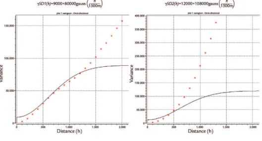
Furthermore, in cases where we do not know any geologic anisotropic pattern a priori, the same variogram model can be used for all categories. Figure 3 shows the experimental variograms and their respective itted models for all ive calcu-lated signed distances. The distances of the experimental variograms never show the nugget effect but it can be arbitrarily added by the user to control the con-nection between the lithologies. In this case a 10% nugget effect was added on all variogram models. All models have
the same range (1500m) and the same proportions between structures contribu-tion (10% for nugget effect and 90% for a Gaussian structure). It can be seen in Figure 3 that the non-stationarity behavior of the distances makes the modelled range somehow arbitrary.
As the absolute value of each var-iogram structure contribution does not affect kriging results, only the propor-tion between the contribupropor-tions, the same variogram model (Equation 13) could be assumed for all ive signed distances.
+
=
m
h
gauss
h
1500
9
.
0
1
.
0
)
(
Now, distances calculated for each category must be interpolated to each grid node, and the category responsible for the most negative estimated distance retained and assigned. Users must input kriging
pa-rameters and variogram models for each lithology. Resolution is the same as the explicit model provided. Grid properties are in Table 2 and kriging parameters are in Table 1; the same kriging parameters
must be used to interpolate all categories. A maximum of 40 samples per estimation makes the run-time a few minutes, the output model differs a little compared to models created using 100 or 200 samples.
Neighborhood Number of samples
Radius (X) Radius (Y) Radius (Z) Min. Samples Max. Samples
Lithology (1-5) 3000m 3000m 3000m 4 40
Number of blocks Block dimensions
Num. X Num. Y Num. Z Dim. X Dim. Y Dim. Z
70 60 57 50m 50m 25m
Table 1
Kriging parameters.
Table 2
Figure 3 Signed distances experimental variograms and their respective models.
A categorical scatterplot, pair-ing each block category deined by the geomodeler, on the X axis, and by the
algorithm, on the Y axis, was constructed (Figure 4) showing a linear correlation coefficient 0.93, namely, 95% of the
Figure 4
Scatterplot of distance function and explicit models, comparing the rock types assigned to each block. Numbers adjacent to the dots refer to quantify of blocks paired.
A high linear correlation coeficient is not indicative of a good model. More simplistic methods such as nearest neighbor also produce highly correlated scattterplots similar to Figure 4; however, produce unrealistic models. In Figure 5, both of the model’s sections were
compared in order to check if interpreted geological structures were reproduced by the algorithm. Slices are vertical along X and Y direc-tions, the block model has 70 sections along the X direction and 60 sections in the Y direction. Four sections along each axis were chosen.
Figure 5
Some complex structures inter-preted by geomodeler were reproduced satisfactorily by the algorithm as can be seen highlighted by green lines (Figure 5). Conversely, the model mathematically generated misses or does not accurately reproduce some other structures, as seen highlighted by red lines (Figure 5), usu-ally, because there were not enough samples in that region, in those cases the geomodeler counted with his/her experi-ence and/or additional information for creating the explicit model. Discordant blocks are shown in red and are located at lithological transitions. Scattered blocks belonging to lithology 5, displayed at the upper part of implicit model, are the blocks assigned conditioning to data lo-cations, where probably the geomodeler arbitrarily increased its inluence in the explicit model. This feature is not ex-pected to be reproduced by the algorithm, as there are few samples from lithology 5 which are surrounded by many lithology 3 and 4 samples.
A trained professional will never be replaced by an algorithm and implicitly
created models will rarely be inal models, as they must be reined manually. The higher the number of samples, the more the implicit model approximates the ex-plicit model, and in this sense, there is no need for much interference. In the case where samples are scarce, the implicit model serves as a proto model, saving time and effort in the early stages of modeling.
Uncertainty was calculated by soft-max transformation, as the probability of each block belonging to each category in each Figure 5 section. The plug-in default value for the factor that regulates the interrelation among the probabilities is ω=175. Lower ω values create more conservative models.
The Servo system and the magnitude of µ factor are dependent on how much
you trust your declustered data propor-tions. In this case study, applying the servo system makes the model more discordant with the model provided for comparison (not necessarily wrong). Border effects often occur when there is extrapolation in estimates, extending structures exaggerat-edly beyond the limits of the samples. The
servo system can also be used to control the extent of this kind of structure.
The implicit geologic modeling algorithm formulation, description, and implementation should be relatively straightforward. Too complex algorithms will be dificult to implement, explain, and justify in practical settings. McLen-nan (2007) proposed six different criteria to evaluate implicit modeling algorithms: (1) Simplicity: The signed distance al-gorithm is extremely simple, where the only tough step is variogram modeling that can be simpliied using the same isotropic variogram for all categories. Speed: It is quite fast. For the case study example where for a dataset with 9140 samples, the algorithm took a few min-utes to run. (3) Subjectivity: Using the same parameters, the model is perfectly replicated. (4) Flexibility: Incorporating incremental geological data is easy and fast. (5) Uncertainty: The transforma-tion of distances in probabilities creates a heuristic measure of uncertainty. (6) Realistic: The algorithm generates geo-logically plausible boundary models.
5. Conclusions
As could be observed in the case study, the algorithm does not replace a trained professional, but its simplicity and speed justify its usage, especially in the early stages of modeling.
As disadvantages of the method, the non-stationarity of the distances can be
mentioned, making the variogram model-ing arbitrary and questionable. Moreover the method is based on kriging, so only linear relationships between domains are modeled, unless a large amount of data is available.
For practical purposes, the heuristic
measure of uncertainty is satisfactory, but it is not an assessment of uncertainty that result from multiple realizations of a sto-chastic model. Knowing this, future work may be focusrd on combining some kind of boundary simulation with the straight-forwardness of the deterministic method.
References
CHILÈS, J et al. Modelling the geometry of geological units and its uncertainty in 3D from structural data: the potential-ield method. In: PROCEEDINGS OF INTER-NATIONAL SYMPOSIUM ON OREBODY MODELLING AND STRATEGIC MINE PLANNING, Perth, Australia, 2004. p. 24.
COWAN, E. J. et al. Practical implicit geological modelling. In: INTERNATIONAL MINING GEOLOGY CONFERENCE, 5. 2003. p. 17-19.
DEUTSCH, C V. et al. Geostatistical software library and user’s guide. New York:
Oxford University Press, 1998.
DEUTSCH, C V., WILDE, J. Modeling multiple coal seams using signed distance functions and global kriging. International Journal of Coal Geology, v. 112, p.
87-93, 2013.
GALLI, A. et al. The pros and cons of the truncated Gaussian method. In: GEOSTA-TISTICAL SIMULATIONS. Springer Netherlands, 1994. p. 217-233.
GUARDIANO, F. B., SRIVASTAVA, R. M. Multivariate geostatistics: beyond biva-riate moments. In: Geostatistics Troia’92. Springer Netherlands, 1993. p. 133-144.
HARDY, R. L. Theory and applications of the multiquadric-biharmonic method 20 years of discovery 1968–1988. Computers & Mathematics with Applications, v.
19, n. 8-9, p. 163-208, 1990.
MODE-LING. Proceedings. 1989a.
JOURNEL, A. G., ISAAKS, E. H. Conditional indicator simulation: application to a Saskatchewan uranium deposit. Journal of the International Association for Ma-thematical Geology, v. 16, n. 7, p. 685-718, 1984.
JOURNEL, A. G. Fundamentals of geostatistics in ive lessons. Washington, DC:
American Geophysical Union, 1989b.
MCCULLOUGH, P., NELDER, J. A. Generalized linear models. 1989.
MCLENNAN, J. A. The decision of stationarity. University of Alberta, 2007. (PhD
Thesis).
MCLENNAN, J. A., DEUTSCH, C. V. Implicit boundary modeling (boundsim). Ed-monton: Centre for Computational Geostatistics, 2006.
NEUFELD, C., WILDE, B. A global kriging program for artifact-free maps. CCG Annual Report, v. 7, p. 403-1, 2005.
SAVCHENKO, V. V. et al. Function representation of solids reconstructed from scatte-red surface points and contours. In: Computer Graphics Forum. Blackwell Science
Ltd, 1995. p. 181-188.
SILVA, D. M. A. Enhanced geologic modeling with data-driven training images for improved resources and recoverable reserves. University of Alberta, 2015. (PhD
Thesis).
SINCLAIR, A. J., BLACKWELL, G. H. Applied mineral inventory estimation.
Cambridge University Press, 2002.
STREBELLE, S. Conditional simulation of complex geological structures using multi-ple-point statistics. Mathematical Geology, v. 34, n. 1, p. 1-21, 2002.