AbstrAct: A two-dimensional second-order positivity-preserving inite volume upwind scheme is developed for a semi-coupled algorithm involving the air and droplet low ields in the Eulerian frame, which shares the grid for each phase. Special emphasis is placed on the computational modeling, which is induced from a strongly-coupled algorithm that satisies the strict hyperbolicity and its numerical scheme based on the Harten-Lax-van Leer-Contact solver preserving the positivity to handle multiphase low in the Eulerian frame. The proposed modeling associated with the semi-coupled algorithm including the Navier-Stokes and droplet equations takes into account different boundary conditions on the solid surface for each phase. The veriication and validation studies show that the new scheme can solve the air and droplet low ields in fairly good agreement with the exact analytical solutions and experimental data. In particular, it accurately predicted the maximum value of the droplet impingement intensity near the stagnation region and the droplet impingement area.
Keywords: Computational luid dynamics, Finite volume method, Harten-Lax-van Leer-Contact scheme, Positivity, Multiphase low, Aircraft icing, Supercooled water droplet.
A Computational Modeling for
Semi-Coupled Multiphase Flow in
Atmospheric Icing Conditions
SungKi Jung1
INTRODUCTION
In the atmosphere, an in-light aircrat icing occurs when supercooled water droplets freeze on impact with any part of the external structure of an aircrat during light in icing conditions, such as a cloud (Lynch and Khodadoust 2001). Icing also occurs on wind turbine blades exposed to low temperatures and water droplets (Parent and Ilinca 2011). Such lows can be found in the air-mixed supercooled water droplet ields. Exposure to this condition for a considerable period can be extremely dangerous to aircrat, as the built-up ice can distort the smooth low of air over the wing. his serious aircrat safety concern can be involved in diminishing the wing’s maximum lit coeicient, reducing the angle of attack for maximum lit coeicient, adversely afecting aircrat handling qualities and signiicantly increasing the drag (Lynch and Khodadoust 2001; Bragg et al. 2005). In addition, aircrat accidents due to icing have been occasionally reported in articles. Representatively, the ATR 72 during an En-route is crashed near Roselawn, Indiana, USA, by the loss of controllability due to icing in 1994 (Gent et al. 2000). A prediction how the water droplets impinge on external structure in such cases can be essential to design proper ice protection systems that prevent or remove ices accumulated on these structures (Kind et al. 1998; Ahn et al. 2015). he design of ice protection systems requires knowledge of the local and total impingement intensities in order to determine the heat inputs for removing built-up ice and the extent of the surface area to be protected. Useful data on the local and total impingement intensities can be obtained via icing wind tunnel tests, or state-of-the-art computational luid dynamics (CFD) simulations. Although the icing wind tunnel
1.Universidade Federal do ABC – Centro de Engenharia, Modelagem e Ciências Sociais Aplicadas – Santo André/SP – Brazil.
Author for correspondence: SungKi Jung | Universidade Federal do ABC – Centro de Engenharia, Modelagem e Ciências Sociais Aplicadas | Avenida dos Estados,
5.001 – Bangú | CEP: 09.210-170 – Santo André/SP – Brazil | Email:[email protected]
tests can provide detailed information, they are very expensive and there are scaling limitations of test models due to wind tunnel sizes in most cases. On the other hand, the CFD-based simulations are relatively cheap and can handle icing problems without limitations (Anderson 2000). Therefore, CFD-based simulations have been increasingly spread and have found their way into the main stream of computational methods for obtaining information about droplet impingement. he numerical simulations to predict droplet impingements have been traditionally based on the two approaches of modeling particle transport in CFD simulations, the Eulerian and the Lagrangian approaches. he Eulerian approach treats the particle phase as a continuum and develops its conservation equations on a control volume basis in a similar form as that for the luid phase. he Lagrangian approach considers particles as a discrete phase and tracks the pathway of each individual particle, such as the NASA LEWICE and ONERA codes (Hamed et al. 2005; Wright et al. 1997; Morency et al. 1999; Silveira et al. 2003; Vu et al. 2002). In the Lagrangian formulation, the trajectory of each particle is computed using a force balance equation. Meanwhile, the Eulerian approach is more lexible for three-dimensional complex geometries.
In general, multiphase lows are simulated using the strong coupled algorithm in which each phase is closely interacted. Nevertheless, the multiphase lows around the aircrat lying into the cloud can be simulated using a weakly coupled algorithm, because the mass loading ratio of the bulk density of the droplets over the bulk density of air is on the order of 10–3 under icing
conditions. It means that the efect of droplets in the air low can be ignored. A number of phenomena and forces may be considered while modeling air-droplets lows, but the following assumptions are sensible in an aircrat icing: the spherical droplets without any deformation or breaking; no droplets collision, coalescence or splashing; no heat and mass exchange between the droplets and the surrounding air; turbulence efects on the droplets can be neglected; the only air drag, gravity and buoyancy forces acting on the droplets (Bourgault et al. 2000). his observation can justify a weakly coupled algorithm in which the calculations for each phase can be independently conducted for the atmosphere icing conditions mixed with the air and a supercooled water droplet. This assumption is however valid for steady state simulations. For unsteady state simulations, such as a moving body, the weakly coupled algorithm may not be valid since, at every time step, air solver should provide the time-dependent primitive variables, such as density and velocity of air low, to the droplet solver taking into account the drag and buoyancy of
droplet. In such cases, multiphase lows around the aircrat may be treated in strongly-coupled or semi-coupled manners so that the equations of each phase are interactively solved or the air low afects the droplet low strongly. For the strongly-coupled manner, the full system of equations is based on the strong interactions between the phases divided by volume fractions. Interestingly, the droplet low does not afect the air low due to the aforementioned assumption, mass loading ratio of the bulk density between each low. It results that the multiphase lows on the aircrat icing do not require the strongly-coupled manner for unsteady simulations. In addition, the full system of equations of strongly-coupled algorithm is very complex and requires a lot of computational resource compared with semi-coupled algorithm. Consequently, the semi-coupled algorithm can be an alternative way to simulate the unsteady simulations.
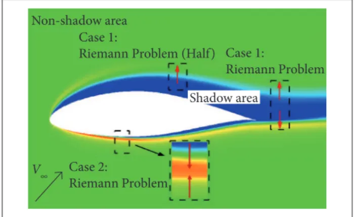
At present, however, critical computational issues remain regarding the CFD-based air-mixed droplet simulations as a uniied solver in which air and droplet solvers are integrated using the single numerical scheme. he issues concern the accuracy of numerical solutions to the droplet equations and its hyperbolic nature. In particular, the liquid water content (LWC) is observed around a solid surface ater the droplets impinge on the surface (Jung and Myong 2013; Jung et al. 2011), as illustrated in Fig. 1. Moreover, it consists of various non-linear wave regions: shock fronts, rarefactions, contact discontinuities, and transitional layers at the interface of the shadow and non-shadow areas. Without proper positivity-preserving schemes, the LWC near the surface may become negative, resulting in the numerical breakdown (Kim et al. 2013). he reason is that the convective system of the droplet equations is not strictly hyperbolic. Even though the system has real eigenvalues, λi = 1, 2, 3= u, they are not distinct and it results that the system of equations does
Figure 1. Liquid water content distribution around an airfoil and identiication of the Riemann problems (Jung and Myong 2013).
Non-shadow area
Shadow area Case 1:
Riemann Problem (Half) Case 1:
Riemann Problem
Case 2:
not satisfy the hyperbolic conservation law. his means that the well-known numerical methods based on the well-posed strictly hyperbolic system such as the approximate Riemann solver may not be applicable, and the special schemes based on the kinetic approximation (Bouchut et al. 2003) are required. To deal with this issue, a two-dimensional second-order positivity-preserving inite volume upwind scheme only for the droplet equations was developed in the previous study (Jung and Myong 2013). he scheme is based on the Harten-Lax-van Leer-Contact (HLLC) approximate Riemann solver (Toro 2001; Toro et al. 1994) for the so-called shallow water droplet model (SWDM) (Jung and Myong 2013). he key component of the scheme is a simple technique based on splitting of the original mathematical system into a well-posed hyperbolic part and the source term in which a vector term involving the divergence of the artiicial term is added and subtracted to the momentum equation for a purely numerical purpose (Jung and Myong 2013).
In this study, a new two-dimensional second-order positivity-preserving inite volume upwind solver for the semi-coupled algorithm in Eulerian frame has been developed using the well-posed hyperbolic part. It will be shown that this numerical scheme satisies the density positivity condition. In addition, the second-order uniied solver of the semi-coupled algorithm in aircrat icing conditions can serve as a basic concept, which is extendable to the moving body simulations. In “Governing Equations” section, the mathematical model of the semi-coupled algorithm for an aircrat icing from a compressible multiphase low (strongly-coupled multiphase algorithm) introduced by Saurel and Abgrall (1999) is reviewed, and the well-posed hyperbolic part of the eigen structure of the system is presented. In “Numerical Methods” section, the second-order finite volume method based on the HLLC approximate Riemann solver is presented. In “Veriication and Validation” section, numerical results of one- and two-dimensional test problems, as the veriication and validation of the new scheme, are presented.
GOVERNING EQUATIONS
Atmospheric multiphase low for an aircrat icing can be treated as a compressible and dilute multiphase low ignoring the droplet efects in air lows since the mass loading ratio of the bulk density of the droplets over the bulk density of air is on the order of 10–3 in lows. Although the lows can be simulated
using a weakly-coupled algorithm for a steady state simulation,
it exposes a limitation for an unsteady state simulation since all primitive variables at every time-marching step cannot be provided into the droplet solver, through the source terms of the droplet equations, due to enormous data size. Consequently, strongly-coupled or semi-coupled algorithms should be employed to simulate unsteady-depended aircrat icing. In this study, the semi-coupled algorithm is proposed by the aforementioned reason in introduction section. he convection-type equations of semi-coupled algorithm for an aircrat icing can be induced by the compressible multiphase low (strongly-coupled algorithm), which is introduced by Saurel and Abgrall (1999). he full system of equations of compressible multiphase low, except for the viscous efects of gas phase and the buoyancy and gravity forces acting on the droplet of liquid phase, is described as:
where:
superscripts g and l denote the gas and liquid phases, respectively; E is the total energy; P means static pressure; I is the identity matrix; V and α are an interfacial velocity and a volume fraction, αg + αl = 1; ρ and u are the density and velocity of each phase, respectively; µ is the viscosity; λ refers to the drag coefficient. The subscript i means an interface between two phases. Using the aforementioned assumptions (αg ~ 1, αgρg = ρ
a, αlρl = ρ
d = LWC, ρ
lPl = 0 and V
i = Pi = 0), the system of equations are summarized as:
(1)
(2)
where:
–λ(ul – ug) denotes a drag force of droplet due to the air low; the subscripts a and d represent the air and the droplet, respectively.
where:
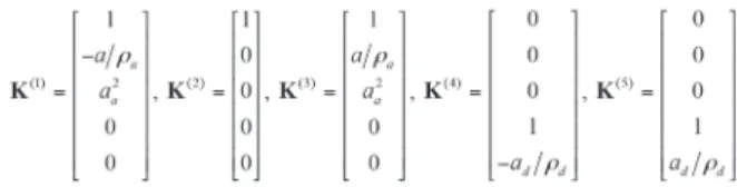
aa is a sound of speed of air low. he matrix A(W) has real eigenvalues, λ1 = ua – aa, λ2 = ua, λ3 = ua + aa, λ4 = λ5 = ud , with corresponding right eigenvectors:
(3)
(5)
(6) (4)
where:
Here, the non-conserved variables τ and Q denote the viscous shear stress tensor and the heat lux, respectively. In Eq. (3), the symbol [Vua](2) in the viscous shear stress tensor stands
for the traceless symmetric part of the tensor; k is the thermal conductivity and depend on the air temperature. For the air low, the ideal equation of state p = ρRT is used in order to close the equations. Sb = ρg[0, 0, 1 – ρa/ρw]T, being ρ
a and ρw the density of air and water, is the resultant force of the gravity and buoyancy of droplets. he Au(ua - ud) denotes the drag acting on droplets caused by the airlow, and g is acceleration due to gravity. Also, the MVD is the mean volume diameter of the droplet. Reu and CDu are the Reynolds number of droplets and the drag coeicients of the spherical droplets, respectively. he drag coeicient can be obtained from Lapple (1951) as follows:
which is valid for Reu < 1,000. In Eq. (3), the first three equations are the well-known Navier-Stokes equations for air low and the last two equations are the droplet equations for droplet low, respectively.
semi-coupled Algorithm with shAllow wAter droplet model for strict
hyperbolicity
A shallow water droplet model based on the Eulerian framework developed in the previous work (Jung and Myong 2013) was employed for the present semi-coupled algorithm. In the present semi-coupled algorithm of Eq. (3), the strict hyperbolic conservation law is not satisied due to a lack of distinctive eigen systems. It means that the well-posed numerical schemes based on the approximated Riemann solvers may not be applied to the equations. In this study, the eigen systems of convective luxes of Eq. (3) are introduced using the primitive formulation of a one-dimensional semi-coupled algorithm in order to proof the lack of distinctive eigen systems:
Even though the matrix A(W) has real eigenvalues, fourth and ith eigenvalues and eigen vectors exactly corresponding to droplet equations are not distinctive. hus, the formulation based on splitting of the droplet equations into the well-posed hyperbolic part and the source term, which circumvents the non-strictly hyperbolic nature of the droplet equations, is applied. he modiied full system of equations involving the previous study can be written as:
and its primitive form with corresponding eigen systems is summarized as:
Wt + A(W)Wx = 0
Wt + A(W)Wx = 0
(7)
ad is (gD)1/2. D and g are a diameter named by the MVD
of droplet and gravity, respectively. he matrix A(W) has real eigenvalues, λ1 = ua – a, λ2 = ua, λ3 = ua + a, λ4 = ud – ad, λ5 = ud + ad , with corresponding right eigenvectors:
here are six distinct waves for the well-posed hyperbolic part of Eqs. 6 and 7. he solutions in the Star region for each phase consist of two constant states separated from each other by a middle wave of speed. In the exact Riemann solver, the middle wave speed S* can be estimated for the particle velocity in the middle state (S* = u*; S is a wave speed and u* is the x-directional particle velocity in the middle state). he well-posed hyperbolic part of governing equations in two-dimensional and x-spirit case can be rewritten as follows with a change of notation ψ = v (v is the y-directional particle velocity):
he tangential velocity component ψ(x, t) represents the concentration of a pollutant or some other passive scalar. he convective lux of Eq. 8 has real and distinct eigenvalues, λ1 = ua – aa, λ2 = λ3 = ua, λ4 = ua + a, λ5 = ud – ad, λ6 = ud, λ7 = ud + ad. he quantity ψ for each phase gives rise to the middle eigenvalue, λ3 = ua and λ6 = ud, respectively. For this hyperbolic system, the following HLLC lux for the approximated Godunov method can be deined at the interface of let and right cells as:
SLa
SRa
S*
t
x
a
S*d
S
R d
URa
U
R d
U
*R a
U
*L a
U*Ld U
*R d
U
L a
ULd
SLd
Figure 2. The HLLC approximate Riemann solver for the well-posed hyperbolic part of the semi-coupled algorithm.
Note that Eqs. 6 and 7 satisfy the hyperbolic conservation law. In the following section, a numerical method is described using the semi-coupled algorithm based on Eqs. 6 and 7.
NUMERICAL METHODS
hllc ApproximAted riemAnn solver for the semi-coupled Algorithm
For the semi-coupled algorithm, a vacuum state caused by the rarefaction waves traveling in opposite directions is analogous to the shadow area, which refers to the very low density of the droplets around a solid surface ater the droplets impinge on the solid surface. Although various numerical methods for preserving the positivity and avoiding the negative density have been published in the past, only a few methods satisfy the positivity in a vacuum state. In particular, the HLLC approximate Riemann solver developed by Toro (2001) and Toro et al. (1994) has shown good behavior and satisies the positivity. In fact, the HLLC approximate Riemann solver for droplet equations can be archived in two- or three-dimensional cases because the HLLC solver basically requires at least three equations to complete wave structures relecting let, right and shear waves. For this reason, a two-dimensional architecture for the semi-coupled algorithm is derived.
Figure 2 illustrates the assumed wave structure in the HLLC approximate Riemann solver for the semi-coupled algorithm.
(8)
(9)
(10)
Ut + F(U)x = 0
where:
where:
wave speeds, SL and SR (L and R subscripts denote the let and right states, respectively), for air lows, employ the direct wave speed estimation, as suggested by Davis (1988), which is the most well-known approach for estimating bounds for the minimum and maximum signal velocities in the solution of the Riemann problem:
and, for droplet,
Even though the minimum and maximum principals for wave speed estimations of let and right sides in Eq. (11) can be imposed to droplet equations, the principals may not ensure the positivity of density in a vacuum state. For this issue, the depth positivity condition proposed by Toro is applied to circumvent numerical diiculties via an assumption of density in a star region:
In Eq. 12, qw is deined by:
where:
ρd
* is an estimate of the exact solution for ρd in the star region. From the depth positivity condition, ρ* in the star region is derived as follows:
he middle wave speeds (S*) in the HLLC Riemann solver are based on the Rankine-Hugoniot conditions across each of the waves, which are basically assumed that all wave speeds are known. he speeds S*, purely in terms of the speeds SL and SR, deined in Eqs. 11 and 12 for each phase, can be expressed as:
for air,
In order to enhance the accuracy, Monotone Upstream Scheme for Conservation Law (MUSCL) proposed by van Leer (1979) together with van Albada limiter (van Albada et al. 1982) is employed:
where:
W = [ρa, ua, ψa, Pa, ρd, ud, ψd]T denotes primitive variables.
The van Albada limiter is defined as ΨL/R = 0.5[(1 + κ)rL/R + (1 – κ)]ФL/R and Ф(r) = 2r/(1 + r2). κ represents an
extrapolation parameter and rR = (Wi+1 – Wi)/(Wi+2 – Wi+1) and rL = (Wi+1 – Wi)/(Wi – Wi-1). A general procedure to precisely solve the Riemann problem for two-dimensional and x-split air and droplet equations is referenced in Toro’s work for air lows and previous work for the shallow water droplet model (Jung and Myong 2013), respectively.
two-dimensionAl finite volume formulAtion
The present finite volume formulation for the semi-coupled algorithm is based on a cell-centered scheme and structured grid. The complete set for the two-dimensional semi-coupled algorithm can be written as:
(11)
(12)
(13)
(14) (18)
(15)
(16)
(17)
where:
where:
dΩ represents the bounding surface of the control volume Ω. he two-dimensional inite volume formulation in general non-Cartesian domains can be derived by exploiting the rotational invariance property of the droplet equations, cosθF(U) + sinθG(U) = T–1F(TU), where T = T(θ) represents
the rotation matrix. Eqs. 18 can then be expressed as:
In the two-dimensional inite volume formulation, the line integral dl on the right-hand side can be approximated by a sum of the luxes crossing the faces of the control volume. It is usually assumed that the lux is constant along the individual interface and is evaluated at the mid-point of the interface. Finally, the following discretized equation is:
he value of droplet density at the interface in source terms is determined as follows:
he air low indeed should take into account viscous efects. In this study, the Spalart-Allmaras turbulence model is employed to simulate the turbulent efect in air low ields and an ideal state of equation is used to close the system of equations.
boundAry conditions
A collection efficiency, a main feature in the in-flight and atmospheric icing, is determined by the droplet density and velocity near the solid surface. It is the fraction of the liquid water, which is deposited as ice on that component while lying in icing conditions. herefore, the setting of the numerical boundary condition on the solid surface is an important factor in solving droplet low ields. When the projection of a normal vector on a solid surface and the droplet velocity in an adjacent cell on the solid surface are positive, the droplets should not collide with the solid surface. On the contrary, when the projection is negative, the droplets should collide with the solid surface. On the basis of this observation, the following simple boundary conditions used in the previous study (Jung and Myong 2013) can be imposed for the droplet size less than 40 μm (see Fig. 3):
(19)
(20)
(21)
(22)
In Eq. 19, the numerical lux Hk at k-th interface is determined by the HLLC approximate Riemann solver. Although the implementation of explicit schemes is much easier than that of implicit schemes, explicit schemes require careful time step selection in order to fulill the stability requirement. he semi-coupled algorithm in this study is calculated under the maximum allowable time steps used in the work of Erduran et al. (2002). he local time stepping for the temporal discretization is achieved using the ith stage Runge-Kutta scheme. In case of unsteady simulation, the minimum time step, ater convergences for each phase, should be chosen to guarantee the stability for each phase.
where:
n = (nx, ny) denotes the normal vector of the solid surface. For the boundary conditions on the solid surface of air lows, a non-slip condition is applied. For the far-ields, Riemann invariant conditions for each phase are applied.
VERIFICATION AND VALIDATION
Two types of problems are selected to verify and validate the second-order positivity-preserving inite volume upwind
V V
Figure 3. Permeable wall boundary condition for droplet impingement (Jung and Myong 2013).
scheme of the semi-coupled algorithm for air-mixed droplet low. he irst problem is intended to compare the exact analytical and numerical solutions as a veriication study. he second problem is the air-mixed droplet low around an airfoil taken from Morency et al. (1999) as a validation study. he conditions, which represent the shadow (very low density of droplet) and high LWC (very high density of droplet) regions in Fig. 1, as the Riemann problems, for the irst problem are summarized in Table 1. The exact and numerical solutions to the one-dimensional well-posed hyperbolic part of the semi-coupled algorithm are compared in Figs. 4 and 5. he computational domain size 50 and 100 grid points with the CFL number 0.2 are used in these computations. Figure 4 (case 1) shows the positivity, which is most vulnerable to the negative density, between two identical rarefaction waves traveling in opposite directions. he HLLC scheme satisies the density positivity condition of droplet; the density of droplet remains very low but always positive in the vacuum region. he new scheme is found to be very accurate for resolving rarefaction waves. he gap in the velocity of droplet is, nonetheless, found in the vicinity of the very low density of droplet. he numerical reason behind this shortcoming for the HLLC scheme is well understood (Toro 2001) and, under the more pressing need of the positivity property, the issue is let for future study. Another Riemann
test cases phase ρl ul pl ρr ur pr time (s) x0
1 Air 1.0 -0.5 1.0 1.0 0.5 1.0 0.3
0.5
Drop 0.0001 -0.5 - 0.0001 0.5
-2 Air 1.0 0.5 1.0 0.5 -0.1 1.0 0.2
Drop 0.0001 0.5 - 0.00005 -0.1
-Table 1. The veriication cases where x0 and t represent the position of the initial discontinuity and the output time in seconds,
respectively. Rarefaction (case 1) and shock (case 2) waves traveling in opposite directions.
problem (case 2) and its numerical solutions are illustrated in Fig. 5. he case is considered in order to investigate the evolution of non-linear waves ater the collision of two streams, which represents the local high LWC region around a leading edge of an airfoil where droplets of the free stream collide with the solid surface. It is clearly shown in Fig. 5 that the density of droplet increases drastically in the star region, indicating a locally high LWC region. he new scheme for this case is found to be very accurate in predicting the shock location and resolving the shock discontinuities. Prior to validate the new scheme for air-mixed droplet low in the in-light and atmospheric icing conditions, the grid sensitivity tests for the new scheme have been conducted by using the ine and coarse grids. Figures 6 and 7 show the grid topologies and convergence histories, respectively. he coarse grid requires less iteration than the ine grid; however, the accuracy due to grid topologies shows that the pressure coeicient of ine grid is more accurate than the coarse grid in Fig. 8. Nevertheless, the new scheme shows the robust characteristics with regard to the grid topologies. In order to validate the new scheme, experimental test cases are selected from the literature (Morency et al. 1999; Silveira et al. 2003; Vu et al. 2002). From the literature survey, the local collection eiciency is deined as the normalized inlux of droplets at a given location, β = –ρdVd/ρd,∞Vd,∞ (Bourgault et al. 1999), where the velocity
Figure 4. The HLLC and the exact solutions of the density and velocity of each phase. Air (a and c); Droplet for semi-coupled algorithm – test case 1 (b and d).
0.0 0.6 0.7 0.8 0.9 1.0 1.1
0.5 x/L
D
en
sit
y
1.0
0.5 1.0
x/L
V
el
o
ci
ty
V
el
o
ci
ty
0.0
0.0E+00 2.0E–05 4.0E–05 6.0E–05 8.0E–05 1.0E–04 1.2E–04
0.2 0.4 0.6 0.8 x/L
LW
C
1.0
0.2 0.4 0.6 0.8 1.0
–0.6 –0.4 –0.2 0.0 0.4
0.2 0.6
–0.6 –0.4 –0.2 0.0 0.4
0.2 0.6
x/L
Present Exact
0.0 0.0 0.2 0.4 0.6 0.8 1.0 1.2
0.5 x/L
D
en
sit
y
1.0
0.5 1.0 0.2
x/L
V
el
o
ci
ty
V
el
o
ci
ty
0.0 0.0E+00 5.0E–05 1.0E–04 1.5E–04 2.0E–04 2.5E–04 3.0E–04
0.2 0.4 0.6 0.8 x/L
LW
C
1.0
0.4 0.6 0.8 1.0
x/L –0.6
–0.4 –0.2 0.0 0.4
0.2 0.6
–0.6 –0.4 –0.2 0.0 0.4
0.2 0.6
Present Exact
magnitude V is determined by a scalar product (ud∙nx + vd∙ny). hus it can quantitatively measure the potential of droplets to collect and the subsequent ice accretion, since the collection eiciency plays an essential role in understanding the droplet impingement and in designing ice protection systems. he test model is a NACA 0012 airfoil with 0.9144 m of cord. he free-stream low velocity is 44.39 m/s and the angle of attack is 0°. he LWC is 0.78 g/m3, the free-stream temperature is 265.5 K and
the MVD of the droplets is 20 µm. he MVD values are assumed to have a monodisperse distribution instead of a Langmuir distribution. he test data is a log-normal distribution itting the original wind tunnel data. For the numerical simulation, a structured grid with an O-type topology and a size of 200 × 74
Figure 5. The HLLC and the exact solutions of the density and velocity of each phase. Air (a and c); Droplet for semi-coupled algorithm – test case 2 (b and d).
Figure 6. Mesh topologies (a) 421 x 65; (b) 150 x 35.
Figure 7. Convergence graphs for ine (a) and coarse grid (b), and the convergence limit for each variable is equal to 10-3.
rho: density.
0 1.0E–04 1.0E–03 1.0E–02
rho u v E
1.0E–01 1.0E+00
50 100
Interations Coarse grid
R
es
id
u
al
s
150 200 250
0 1.0E–04 1.0E–03 1.0E–02 1.0E–01 1.0E+00
100 200 Interations
Fine grid
R
es
id
u
al
s
300 400 250
(b) (b)
(a) (a)
are used. Figure 9 shows the structure mesh distribution around the NACA0012 airfoil and the mesh near the solid surface are clustered to capture viscous efects. Figure 10 shows the distributions of pressure coeicient and the collection eiciency on the solid surface for each phase, respectively. he present computational results of each phase are in close agreement with experimental data, demonstrating that the present semi-coupled algorithm code is capable of producing the air and droplet information. Figure 11 shows the pressure and LWC distributions around the test model with an angle of attack
of 0.0°. In particular, a very low density of LWC is shown in the shadow area near the upper and lower side of the airfoil. he area of shadow zone at both the upper and lower sides of the airfoil is almost the same, mainly due to the efect of the free stream angle of attack and symmetrical shape. Furthermore, in order to check the low LWC results compared with free stream low LWC, the low LWC values in the shadow area around the middle point of airfoil are presented in Fig. 12. In the shadow areas, the low LWC values show the 1.4465e–05 g/m3
and 7.3195e–06 g/m3 around the upper and lower surfaces,
respectively. hose values are less than 0.0002% compared with the free stream low LWC.
Figure 8. Comparisons of ine and coarse grids with the experiment data.
–0.8
–0.4
0
0.4
0.8
1.2
0 0.2 0.4
x/L NACA65(2)415
Experiment Fine
Coarse
Cp
0.6 0.8 1
0 0.2 0.4
–0.4 –0.2 0 0.2 0.4
x
y
0.6 0.8 1
–10 –5 0
–10 –5 0 5 10
x
y
5 10
0 0.2 0.4
–0.4 –0.2 0 0.2
0.4 LWC:1E–053E–05 5E–05 7E–05 9E–05
x
y
0.6 0.8 1
0 0.2 0.4 0.6
–0.4 –0.2 0 0.2 0.4
x
y
0.8 1
–0.4 –0.2 0 0.2 0.4 0.6 0.8 Cp:
–0.1 –0.05
C
o
ll
ec
ti
o
n
e
ffi
ci
en
cy
0.05 0.1 0
S [m] Lower Upper
0 0.1 0.2 0.3 0.4 0.5 0.6
Cp
x/L
1.2 1.0 0.6
0.8 0.4 0.2
0.0 0.5 1.0
Experiment Present –0.6
–0.4
–0.4
Cp: pressure coeficient.
Figure 9. Far ield (a) and clustered (b) grid distributions near the NACA0012 airfoil.
Figure 10. Present and experimental results of pressure coeficient (a) and collection eficiency (b) for the NACA 0012.
Figure 11. Pressure coeficients (a) and LWC (b) distributions around NACA 0012 airfoil.
(b) (b)
(a)
(a)
(b)
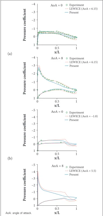
Figure 13. Pressure distributions on the surfaces of MS-0317 (a) and NLF-0414 (b) Airfoils.
AoA: angle of attack. Also, the validation tests are extended and simulated via
the existing experimental results, which are conducted by the NASA in USA, in order to compare the present results, including other existing codes, which are provided from the literature (Vu et al. 2002). In particular, the efects of higher angles of attack, diferent droplet sizes and airfoil shapes are presented and the test conditions are summarized in Table 2. Figure 13 shows the pressure coeicients on the surfaces of MS-0317 and NLF-0414 airfoils. In case of the LEWICE, the angles of attack in computations were slightly adjusted by approximately –2.0° to 2.5° depending on the test model, in order to match the experimental pressure. he proposed method, however, does not match the experimental pressure. Nevertheless, the present results are in relatively good agreement with experimental results. Figure 14 shows the efects of higher angles of attack of the MS-0317 airfoil with other ixed test conditions. he droplet impingement limits are moved from the upper surface to the lower surface around a leading edge, and maximum impingement intensities are slightly decreased in case of an angle of attack of 8°. Regarding the MVD efects, the maximum impingement intensity and droplet impingement limit are proportional to the size of droplet diameters. Figure 15 clearly shows that small droplet size is less efective than the large droplet size. Figures 16 and 17 present the airfoil shape efects with other ixed test conditions. In fact, the shape efects may be considered as an inluence of the leading edge radius shown in Fig. 16, where the MS-0317 airfoil has a larger leading-edge
test model Angle of attack (°) velocity (m/s) chord (m) mvd (μm) lwc (g/m3) re (1.0e+6) MS-0317
0; 0.8 78.66 0.9144 11; 21.5 0.04; 0.15 4.83
NLF-0414
Table 2. Test models and conditions.
Figure 12. The low LWC values around middle points of upper and lower sides of the NACA0012 airfoil in the shadow area.
0.4 0.45 –0.05 0 0.05 0.1 0.5 7.3195E-11 1.4465E-10 x y 0.55 –5 –4 –3 –2 –1 0 0 0.5 x/L P ress u re c o e ffi ci e n t 1 1 –5 –4 –3 –2 –1 0 0 0.5 x/L P r ess ur e c o e ffi ci e n t 1 1 –4 –3 –2 –1 0 0 0.5 x/L P r ess ur e c o e ffi ci e n t 1 1 –4 –3 –2 –1 0 0 0.5 x/L AoA = 0
AoA = 8
AoA = 0
AoA = 8
P r ess ur e c o e ffi ci e n t 1 1 Experiment
LEWICE (AoA = 6.15) Present
Experiment
LEWICE (AoA = –1.0) Present
Experiment
LEWICE (AoA = 5.5) Present
Experiment
LEWICE (AoA = 6.15) Present
radius than the NLF-0414 airfoil. It results that the maximum impingement intensity is decreased, and the impingement limit is increased, inversely.
(a)
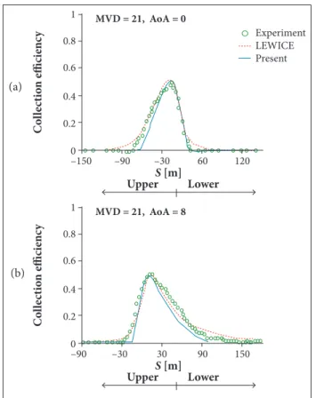
Figure 14. Effects of higher angle of attack of the MS-0317 airfoil. –90 0 0.2 0.4 0.6 0.8
1 MVD = 21, AoA = 8
–30 30 90 150
Lower Upper C o lle ct io n e ffic ie n cy
S [m] –150 0 0.2 0.4 0.6 0.8
1 MVD = 21, AoA = 0
–90 –30 60 120
Experiment
LEWICE Present Lower Upper C o lle ct io n e ffic ie n cy
S [m]
–120 0 0.2 0.4 0.6 0.8
1 MVD = 21, AoA = 0
–60 30 90 150
Lower Upper C o lle ct io n e ffic ie n cy
S [m] –150 0 0.2 0.4 0.6 0.8
1 MVD = 21, AoA = 0
–90 –30 60 120
Experiment
LEWICE Present Lower Upper C o lle ct io n e ffic ie n cy
S [m]
MS-0317 NLF-0414 –120 0 0.2 0.4 0.6 0.8
1 MVD = 11, AoA = 0
–60 0 60 120
Lower Upper C o lle ct io n e ffic ie n cy
S [m] –150 0 0.2 0.4 0.6 0.8
1 MVD = 21, AoA = 0
–90 –30 60 120
Experiment LEWICE Present Lower Upper C o lle ct io n e ffic ie n cy
S [m]
Figure 15. MVD effects of the MS-0317 airfoil.
Figure 16. Different airfoil shapes. MS-0317 and NLF-0414 airfoils.
CONCLUSIONS
A semi-coupled algorithm was proposed and its
two-dimensional second-order positivity-preserving finite volume upwind solver was developed for the semi-coupled algorithm of air and droplet flows in atmospheric icing conditions. Much attention was paid to the mathematical descriptions of semi-coupled algorithm and preservation of density positivity in the numerical scheme, as well as the verification and validation study of the scheme. From the previous study (Jung and Myong 2013), the positivity-preserving property was achieved by the splitting of the original mathematical Figure 17. Airfoil shape effectiveness. MS-0317 (a) and NLF-0414 (b) airfoils.
system into the well-posed hyperbolic part and the source term and then applying the positivity-preserving HLLC approximate Riemann solver to the semi-coupled algorithm. In the veriication and validation studies, it was shown that the new scheme can solve the air and droplet low ields in fairly good agreement with the exact analytical solutions and experimental data, respectively. For the veriication, the vacuum state and the shock wave due to two rarefaction waves and the collision of two waves were tested. In particular, a shock wave due to the collision of two waves could be considered as a droplet path line intersection, which represents the locally high LWC region around a leading edge of an airfoil where droplets of the free stream collide with the solid surface. It is clearly shown in Fig. 5 that the density of droplet increases drastically in the star region, indicating a locally high LWC region. he new scheme for this case is found to be very accurate in comparisons of exact solutions with the shock location and the shock discontinuities. In addition, Fig. 11 shows the locally high LWC distributions around the leading edge of the airfoil. From Figs. 5 and 11, the present scheme for the droplet path line intersection may circumvent the local accuracy limitations due to the numerical instability in the Eulerian framework. For the
validation, various test models were chosen and the new scheme showed the applicability for air-mixed in-light icing conditions in comparisons of existing wind tunnel droplet impingement test results. In particular, it accurately predicted the maximum value of the droplet impingement intensity near the stagnation region and the droplet impingement area. Such capability may be due to the second-order accuracy of numerical scheme in spatial discretization, while satisfying the positivity-preserving requirement. It should be noted that, without proper positivity-preserving schemes, to slow the appearance of breakdown due to negative density, the numerical code should remain irst-order instead of second-irst-order, typical in CFD, which in turn may cause the underprediction of impingement intensity near the stagnation region.
In this study, a construction of the semi-coupled algorithm and its numerical approaches were mainly considered; nonetheless, there is still a room of improvement in the computational modeling of the moving body techniques for unsteady simulations. For example, periodically up and down motions of airfoils in order to simulate a section of helicopter rotor blades. he study of the problem will be the subject of a future paper.
REFERENCES
Ahn GB, Jung KY, Myong RS, Shin HB, Habashi WG (2015) Numerical and experimental investigation of ice accretion on a rotorcraft engine air intake. J Aircraft 52(3):903-909. doi: 10.2514/1.C032839
Anderson DN (2000) Effect of velocity in icing scaling tests. AIAA-2000-0236.
Bouchut F, Jin S, Li X (2003) Numerical approximations of pressureless and isothermal gas dynamics. SIAM J Numer Anal 41(1):135-158. doi: 10.1137/S0036142901398040
Bourgault Y, Boutanios Z, Habashi WG (2000) Three-dimensional Eulerian approach to droplet impingement simulation using FENSAP-ICE, Part 1: model, algorithm, and validation. J Aircraft 37(1):95-103. doi: 10.2514/2.2566
Bourgault Y, Habashi WG, Dompierre J, Baruzzi GS (1999) A inite element method study of Eulerian droplets impingement models. Int J Numer Meth Fluids 29(4):429-449. doi: 10.1002/(SICI)1097-0363(19990228)29:4<429::AID-FLD795>3.0.CO;2-F
Bragg MB, Broeren AP, Blumenthal LA (2005) Iced-airfoil aerodynamics. Prog Aerosp Sci 41(5)323-362. doi: 10.1016/ j.paerosci.2005.07.001
Davis SF (1988) Simpliied second-order Godunov-type methods. SIAM J Sci Stat Comput 9(3)::445-473. doi: 10.1137/0909030
Erduran KS, Kutija V, Hewett CJM (2002) Performance of inite
volume solutions to the shallow water equations with shock-capturing schemes. Int J Numer Methods Fluids 40(10):1237-1273. doi: 10.1002/ld.402
Gent RW, Dart NP, Cansdale JT (2000) Aircraft icing. Phil Trans R Soc Lond A. 358:(1776)2873-2911. doi: 10.1098/rsta.2000.0689
Hamed A, Das K, Basu D (2005) Numerical simulation of ice droplet trajectories and collection eficiency on aero-engine rotating machinery. AIAA-2005-1248.
Jung SK, Myong RS (2013) A second-order positivity-preserving inite volume upwind scheme for air-mixed droplet low in atmospheric icing. Comput Fluids 86:459-469. doi: 10.1016/j.compluid.2013.08.001
Jung SK, Myong RS, Cho TH (2011) Development of Eulerian droplets impingement model using HLLC Riemann solver and POD-based reduced order method. AIAA-2011-3907.
Kim JW, Dennis PG, Sankar LN, Kreeger RE (2013) Ice accretion modeling using an Eulerian approach for droplet impingement. AIAA-2013-0246.
Kind RJ, Potapczuk MG, Feo A, Golia C, Shah AD (1998) Experimental and computational simulation of in-light icing phenomena. Prog Aerosp Sci 34(5-6):257-345. doi: 10.1016/S0376-0421(98)80001-8
Lynch FT, Khodadoust A (2001) Effects of ice accretions on aircraft aerodynamics. Prog Aerosp Sci 37(8):669-767. doi: 10.1016/ S0376-0421(01)00018-5
Morency F, Tesok F, Paraschivoiu I (1999) Anti-icing system simulation using CANICE. J Aircraft 36(6):999-1006. doi: 10.2514/2.2541
Parent O, Ilinca A (2011) Anti-icing and de-icing techniques for wind turbines: critical review. Cold Reg Sci Technol 65(1):88-96. doi: 10.1016/j.coldregions.2010.01.005
Saurel R, Abgrall R (1999) A multiphase Godunov method for compressible multiluid and multiphase lows. J Comput Phys 150(2):425-467. doi: 10.1006/jcph.1999.6187
Silveira RA, Maliska CR, Estivam DA, Mendes R (2003) Evaluation of collection eficiency methods. Proceedings of the 17th International Congress of Mechanical Engineering; São Paulo, Brazil.
Toro EF (2001) Shock-capturing methods for free-surface shallow lows. Chichester: Wiley.
Toro EF, Spruce M, Speares W (1994) Restoration of the contact surface in the HLL-Riemann solver. Shock Waves 4(1):25-34. doi: 10.1007/BF01414629
van Albada GD, van Leer B, Roberts Jr WW (1982) A comparative study of computational methods in cosmic gas dynamics. Astron Astrophys 108(1)::76-84. doi: 10.1007/978-3-642-60543-7_6
van Leer B (1979) Towards the ultimate conservative difference scheme V. A second order sequel to Godunov’s method. J Comput Phys 32(1):101-136. doi: 10.1016/0021-9991(79)90145-1
Vu GT, Yeong HW, Bidwell CS, Breer MD, Bencic TJ (2002) Experimental investigation of water droplet impingement on airfoils, inite wings, and an S-duct engine inlet. NASA/TM-2002-211700.