Article
Crop Monitoring Based on SPOT-5 Take-5 and
Sentinel-1A Data for the Estimation of Crop
Water Requirements
Ana Navarro1,*, João Rolim2, Irina Miguel3, João Catalão1, Joel Silva4, Marco Painho4 and Zoltán Vekerdy5
1 IDL, Departamento de Engenharia Geográfica, Geofísica e Energia, Faculdade de Ciências,
Universidade de Lisboa, 1749-016 Lisboa, Portugal; jcfernandes@fc.ul.pt
2 LEAF, Departamento de Ciências e Engenharia de Biossistemas, Instituto Superior de Agronomia,
Universidade de Lisboa, 1349-017 Lisboa, Portugal; joaorolim@isa.ulisboa.pt
3 Departamento de Geologia, Faculdade de Ciências, Universidade Agostinho Neto, 1231 Luanda, Angola;
ilfmiranda@hotmail.com
4 NOVA IMS, Information Management School, Universidade Nova de Lisboa, 1070-312 Lisboa, Portugal;
jsilva@novaims.unl.pt (J.S.); painho@novaims.unl.pt (M.P.)
5 ITC, Department of Water Resources, Faculty of Geo-information Science and Earth Observation,
University of Twente, P.O. Box 6, 7500 AA Enschede, The Netherlands; z.vekerdy@utwente.nl
* Correspondence: acferreira@fc.ul.pt; Tel.: +351-217-500-830
Academic Editors: Zhongbo Su, Yijian Zeng, Clement Atzberger and Prasad S. Thenkabail Received: 31 March 2016; Accepted: 14 June 2016; Published: 22 June 2016
Abstract:Optical and microwave images have been combined for land cover monitoring in different agriculture scenarios, providing useful information on qualitative and quantitative land cover changes. This study aims to assess the complementarity and interoperability of optical (SPOT-5 Take-5) and synthetic aperture radar (SAR) (Sentinel-1A) data for crop parameter (basal crop coefficient (Kcb) values and the length of the crop’s development stages) retrieval and crop type classification, with a focus on crop water requirements, for an irrigation perimeter in Angola. SPOT-5 Take-5 images are used as a proxy of Sentinel-2 data to evaluate the potential of their enhanced temporal resolution for agricultural applications. In situ data are also used to complement the Earth Observation (EO) data. The Normalized Difference Vegetation Index (NDVI) and dual (VV + VH) polarization backscattering time series are used to compute theKcbcurve for four crop types (maize, soybean, bean and pasture) and to estimate the length of each phenological growth stage. TheKcbvalues are then used to compute the crop’s evapotranspiration and to subsequently estimate the crop irrigation requirements based on a soil water balance model. A significantR2correlation between NDVI and backscatter time series
was observed for all crops, demonstrating that optical data can be replaced by microwave data in the presence of cloud cover. However, it was not possible to properly identify each stage of the crop cycle due to the lack of EO data for the complete growing season.
Keywords: agriculture; land cover change; SPOT-5 Take-5; Sentinel-1A; evapotranspiration; TIGER initiative
1. Introduction
Crop monitoring by satellite remote sensing requires high spatial and temporal resolution image time series and ground campaigns to monitor the entire crop cycle with frequent ground acquisitions over extensive areas. With the ever-increasing number of satellites and the availability of free data, the integration of multisensor images in coherent time series offers new opportunities for land cover and crop type classification [1]. In addition, satellites with a shorter revisit time (e.g., six days at the
Equator for the Sentinel-1 constellation and five days at the Equator under cloud-free conditions for the Sentinel-2 constellation) and reconfigurable acquisitions (different viewing conditions can be applied for more frequent observation of a certain area) can be used to better identify the different growth cycle stages that are often imperceptible when using more sporadic data.
Many studies have combined optical and microwave images to improve mapping accuracy in agricultural scenarios [2–7]. SAR data are independent of solar illumination and depend on the wavelength and on the roughness, geometry and material contents of the targeted surface. In contrast, optical data are greatly influenced by cloud cover and represent the reflectance of solar energy from a target area. The potential of Earth Observation (EO) techniques for the management of land and water resources has also been widely acknowledged [8,9]. The repeatability of observations on a cyclic basis and the availability of high spatial resolution multispectral data are particularly suitable for cost-effectively mapping crops and irrigated areas with satisfactory accuracy [10].
The amount of water required to meet the cropped field’s water loss through evapotranspiration is defined as the crop water requirement [11,12]. Water requirements vary from crop to crop and throughout the growing season of an individual crop. The FAO Penman–Monteith method is the standard method for the definition and computation of the reference evapotranspiration (ETo) [13,14]. Crop evapotranspiration (ETc) from crop surfaces under standard conditions is determined by crop coefficients (Kc) that relateETc to ETo. The dual crop coefficient approach separatesKc into two separated coefficients, one for crop transpiration (Kcb, basal crop coefficient) and another for soil evaporation (Ke).
EO methodologies have been used to estimateETcdue to the reflective properties of vegetation and to the relationship ofETcwith crop characteristics, such as the Leaf Area Index (LAI) and crop coefficient (Kc).ETccan be estimated from EO data using physics-based methods based on the surface energy balance [15–17] or using empirical methods based on the use of vegetation indices [10,18–20]. Physics-based methods estimate latent heat flow through the surface energy balance, but the difficulties related to the measurement of its terms have led to a wider use of the empirical methods, in which the crop coefficient is obtained through the vegetation indices approach. The estimation ofETcbased on vegetation indices, usually the NDVI, is a modification of the crop coefficients method [11,12], in which ETois calculated based on meteorological data, and the crop coefficient introduces information related to the crop. In these methods, crop data are often obtained through tabulated values, which provide general data for several crops [13,14]. To improve the accuracy of crop water requirement estimation, the characterization of theKccurves must be improved and can be done using EO data, because crop characteristics are well correlated with the spectral reflectances [21]. Thus, as proposed by several authors [10,18–20], theKc-NDVI approach establishes an empirical relationship betweenKcvalues obtained through field measurements and NDVI values retrieved from EO optical data. The equations used to estimate crop coefficient values based on vegetation indices, once calibrated and validated for a given location, can accurately estimate crop evapotranspiration [10,21].
2. Materials and Methods
2.1. Test Area
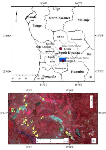
The test area covers an irrigation perimeter close to the town of Wako-Kungo (11˝25133”S, 15˝06110”E), which is located in the Cela Municipality, South-Kwanza Province, Angola (Figure1). The test area has an area of approximately 960 km2, with 40 km in the west-east direction and 24 km in
the north-south direction. The Wako-Kungo region is located on a plateau zone higher than 1200 m. This region has a warm temperate climate with a marked wet season from October to April and an average annual precipitation of approximately 1250 mm. The dry season (Cacimbo) occurs from May to August. The average annual temperature is approximately 21˝C, ranging between 22˝C in September and October and 18˝C in June [23–25].
The Cela area has a dense hydrographic network that is limited by the River Nhia in the north and the River Queve in the south. There is also the River Kusonhi and a large number of streams with appreciable flow during the months of the rainy season that contribute to the available water in the region. This region is dominated by ferralitic soils in association with para-ferralitic soils, which occur in hilly areas, especially in foothills. The area climate conditions combined with the soil types present in the region make the area soils fertile for agriculture. The main crops in the rainy season are maize, rice, some vegetables and pasture, with dairy farming being the main activity. The crops and pastures in this region require irrigation during the dry season [23–25].
′ ″ ′ ″
Figure 1.(a) Regional context of the test area (solid blue rectangle) with the location of the Kibala and
2.2. Data and Field Work
2.2.1. Satellite Data and Preprocessing
To achieve a high temporal resolution, Sentinel-1A and SPOT-5 Take-5 images were requested from ESA (European Space Agency) and from CNES (Centre National d’Études Spatiales), respectively, within the scope of the ESA Alcantara initiative project (Ref: 14-P13) and the SPOT-5 Take-5 project (ID: 29142) for the time period from March to September 2015.
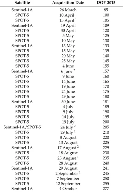
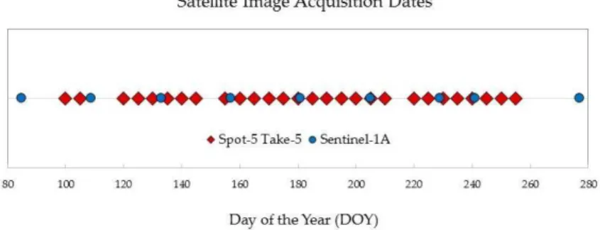
A total of 37 satellite images were made available for this study: 28 SPOT-5 Take-5 images from 10 April to 12 September and 9 Sentinel-1A images from 26 March to 4 October (Table1and Figure2).
Table 1.Sentinel-1A and SPOT-5 Take-5 acquisition dates (day of the year (DOY) 2015).
Satellite Acquisition Date DOY 2015
Sentinel-1A 26 March 85
SPOT-5 10 April1 100
SPOT-5 15 April1 105
Sentinel-1A 19 April 109
SPOT-5 30 April 120
SPOT-5 5 May 125
SPOT-5 10 May 130
Sentinel-1A 13 May 133
SPOT-5 15 May 135
SPOT-5 20 May 140
SPOT-5 25 May 145
SPOT-5 4 June 155
Sentinel-1A 6 June2 157
SPOT-5 9 June 160
SPOT-5 14 June 165
SPOT-5 19 June 170
SPOT-5 24 June 175
SPOT-5 29 June 180
Sentinel-1A 30 June 181
SPOT-5 4 July 185
SPOT-5 9 July 190
SPOT-5 14 July 195
SPOT-5 19 July 200
Sentinel-1A/SPOT-5 24 July2 205
SPOT-5 29 July1 210
SPOT-5 8 August 220
SPOT-5 13 August 225
Sentinel-1A 17 August2 229
SPOT-5 18 August 230
SPOT-5 23 August1 235
SPOT-5 28 August 240
Sentinel-1A 29 August 241
SPOT-5 2 September1 245
SPOT-5 7 September 250
SPOT-5 12 September 255
Sentinel-1A 4 October 277
β σ γ
σ
Figure 2. Sentinel-1A and SPOT-5 Take-5 acquisition timeline, from 26 March 2015 (DOY 85) to
4 October 2015 (DOY 277).
The Sentinel-1 mission comprises a constellation of two polar-orbiting satellites, operating day and night and performing C-band synthetic aperture radar (SAR) imaging, enabling image acquisition regardless of the weather. Sentinel-1A was launched on 3 April 2014, while Sentinel-1B was launched on 25 April 2016. The Sentinel-1A mission includes SAR imaging in four exclusive imaging modes with different resolutions (down to 5 m) and coverages (up to 400 km). This mission provides dual polarization capability, very short revisit times and rapid product delivery. A single Sentinel-1 satellite can potentially map the global landmasses in interferometric wide (IW) swath mode once every 12 days in a single pass (ascending or descending). The two-satellite constellation offers a 6-day exact repeat cycle at the Equator. Because orbit track spacing varies with latitude, the revisit rate is significantly greater at higher latitudes than at the Equator.
All of the Sentinel-1A C-band SAR images were made available in IW mode with a dual polarization scheme (VV + VH). These images were distributed as Level-1 products, as single look complex (SLC), except for the first two acquisition dates, and as ground range detected (GRD) for all dates. SLC image ground resolution is 5 mˆ20 m, while that for GRD images is 10 m. All of the images were acquired in ascending mode with incidence angles ranging from 38.87˝ to 39.26˝. Sentinel-1A Level-1 GRD products were used in this study due to their improved quality. However, because typical SAR data processing, which produces Level-1 images, does not include radiometric corrections and because significant radiometric bias remains, it is necessary to radiometrically correct the SAR images. Moreover, radiometric correction is also required when comparing SAR images acquired from the same sensor, but at different times, as in this study. Radiometric calibration was applied using the following equation (Equation (1)) [26]:
γi“ pDN2
i `bq
Ai (1)
whereAiis the gamma calibration vector(i),bis a constant offset andDNi2is the intensity. Level-1 products provide four calibration look-up tables (LUTs) to produce β0i, σ0i and γi or a digital
number (DN). The LUTs apply a range-dependent gain, including the absolute calibration constant. Independently of the selected LUT (in this case,σ0iwas chosen), for any pixelithat falls between
points in the LUT, theAivalue is found by bilinear interpolation.
A terrain correction was also applied to the images because, due to the topographical variations of a scene and the tilt of the satellite sensor, distances can be distorted in SAR images. The range Doppler orthorectification method was used to geolocate all of the SAR images using available orbit state vector information in the metadata, radar timing annotations, slant-to-ground range conversion parameters and reference DEM data. NASA’s Shuttle Radar Topography Mission (SRTM) DEM sampling at 3 arc-seconds was adopted.
time series were made available to the scientific community by ESA and CNES to support the development of time series analysis in preparation for the exploitation of the Sentinel-2 mission.
Level-2A SPOT-5 images were used in this study due to their improved pre-processing level. The highest quality product (ORTHO_SURF_CORR_PENTE) was chosen because it provides surface reflectances corrected from atmospheric effects (top of atmosphere), including adjacency effects and even terrain effects. Therefore, no further pre-processing steps were required for these images.
2.2.2. Field Work
Crop ground truth information was collected in the field from 15 to 30 April 2015. A total of 56 eligible parcels were mapped during the campaign (see Figure1for parcel location). The crop types identified in the field were mainly maize, but soybean, common (dry) bean (hereinafter designated as bean) and pasture were also observed (Table2). Other crop types observed in the field were not considered in this study due to the small number of plots. The size of the parcels differs significantly, varying from a minimum of 0.43 ha to a maximum of 110.03 ha.
During the field campaign, for each parcel, the crop type and its phenological growth stage according to the BBCH (“Biologische Bundesanstalt, Bundessortenamt und CHemischeIndustrie”) scale [27] were registered. For maize, most of the parcels were in the senescence (Sen) stage, while 1 parcel was in the flowering (Fl) stage and another one in the leaf development (Lf) stage. All of the soybean parcels were in the senescence phase, while for bean, 1 parcel was in Lf; 3 parcels were in Fl; and 1 parcel was in the fruit development (Fr) stage. Pasture is harvested several times during the growing season; therefore, this crop is always in the Lf stage. Whenever possible, the sowing date was also collected for each parcel.
Table 2. Crop type and number of parcels identified in the test area during the field work. Sen,
senescence; Fl, flowering; Lf, leaf development.
Crop Type No. of Parcels Min. Area (ha) Max. Area (ha) Phenological Growth Stage
Maize 28 4.48 110.03 1 Lf, 1 Fl and 26 Sen
Soybean 13 4.47 48.95 Sen
Pasture 5 9.64 14.79 Lf
Bean 5 0.43 42.31 1 Lf, 3 Fl and 1 Fr
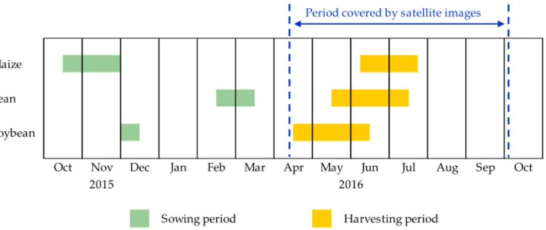
In Figure3, a crop calendar of the main crops observed in the Wako-Kungo irrigation perimeter is presented. These dates are the most common dates for these crops in this region. The sowing and harvesting periods for maize, bean and soybean are shown, while pasture is omitted because it is always in the crop development stage. According to Figure3, the period covered by the satellite images does not cover the entire growing season.
Period covered by satellite images
Maize Bean Soybean
Sowing period Harvesting period
Nov Dec Jan Feb Mar Oct
2015 2016
Apr May Jun Jul Aug Sep Oct
Additionally, the boundaries of each parcel were determined in the field using a GPS receiver, which permitted the creation of a polygon vector file in the WGS84/UTM 33S coordinate reference system. The local weather conditions were recorded at a local weather station (11˝1615711S, 14˝5915011E) managed by the Instituto de Investigação Agrária(IIA). However, a few days after the end of the campaign, the station went out of order and was able to register data again beginning 13 October.
2.2.3. Meteorological Data
Data from the SASSCAL (Southern African Science Service Centre for Climate Change and Adaptive Land Management) WeatherNet [28] were used as input for the soil water balance model. The station nearest to the test area is Wako-Kungo (11˝2414011S, 15˝0714511E, 1331 m in altitude), approximately 20 km southeast of the IIA weather station. However, because data related to air temperature and humidity are lacking until 20 May, data from Kibala (Catofe) station (10˝4411011S, 14˝5910411E, 1272 m in altitude, approximately 60 km north of the IIA weather station) were also downloaded. The location of each station is displayed in Figure1.
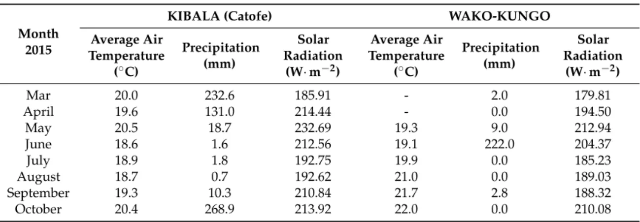
The weather parameters available to calculate the crop water requirements and that were common to both stations were air temperature, precipitation, air humidity and solar radiation. Wind speed, required for the soil water balance model, was only available for Wako-Kungo from 1 March to 18 June. Monthly average air temperature, precipitation and solar radiation values are listed in Table3for the Kibala and Wako-Kungo stations.
Table 3.Monthly average air temperature, precipitation and solar radiation values for the Kibala and Wako-Kungo stations of the SASSCAL WeatherNet.
Month 2015
KIBALA (Catofe) WAKO-KUNGO
Average Air Temperature
(˝C)
Precipitation (mm)
Solar Radiation
(W¨m´2)
Average Air Temperature
(˝C)
Precipitation (mm)
Solar Radiation
(W¨m´2)
Mar 20.0 232.6 185.91 - 2.0 179.81
April 19.6 131.0 214.44 - 0.0 194.50
May 20.5 18.7 232.69 19.3 9.0 212.94
June 18.6 1.6 212.56 19.1 222.0 204.37
July 18.9 1.8 192.75 19.9 0.0 185.23
August 18.7 0.7 192.62 21.0 0.0 189.03
September 19.3 10.3 210.84 21.7 2.8 188.32
October 20.4 268.9 213.92 22.0 0.0 210.08
2.3. Method
2.3.1. NDVI and VV + VH Backscattering Time Series
SPOT-5 Bands B2 (Red) and B3 (NIR) were used to compute an NDVI image for each epoch [29]. Based on these NDVI images, it was possible to calculate the average NDVI and the standard deviation values for each crop parcel. SPOT-5 Take-5 time series graphs for each crop type (pasture, maize, soybean and bean) and for each epoch were generated to assess the behavior of each crop throughout the entire growing season using the trend analysis of the NDVI values.
Likewise, the gamma VV + VH bands were used to determine the mean value for each crop type and for each epoch. After calculating the mean values, they were converted from power scale values into logarithmic scale values to correctly represent dB values using the following equation (Equation (2)):
γipdBq “10ˆlog10pγiq (2)
2.3.2. Image Classification and Accuracy Assessment
Two supervised classification methods were used for image classification: support vector machine (SVM) and neural network (NN).
SVM is a supervised classification method derived from statistical learning theory that often yields good classification results from complex and noisy data [30–32]. It separates the classes with a decision surface that maximizes the margin between the classes. The surface is often called the optimal hyperplane, and the data points closest to the hyperplane are called support vectors. The support vectors are the critical elements of the training set. SVM can be adapted using nonlinear kernels to become a nonlinear classifier. While SVM is a binary classifier in its simplest form, it can function as a multiclass classifier by combining several binary SVM classifiers (creating a binary classifier for each possible pair of classes). SVM includes a penalty parameter that allows a certain degree of misclassification, which is particularly important for non-separable training sets. The penalty parameter controls the trade-off between allowing training errors and forcing rigid margins. It creates a soft margin that permits some misclassifications, such as it allows some training points on the wrong side of the hyperplane. Increasing the value of the penalty parameter increases the cost of misclassifying points and forces the creation of a more accurate model that may not generalize well.
NN applies a layered feed-forward neural network classification technique. The NN technique uses standard backpropagation for supervised learning [33,34]. You can select the number of hidden layers to use and can choose between a logistic or hyperbolic activation function. Learning occurs by adjusting the weights in the node to minimize the difference between the output node activation and the output. The error is back propagated through the network, and the weight is adjusted using a recursive method. NN classification can be used to perform non-linear classification.
To evaluate the potential of integrating microwave data with optical data into the classification process, the following pairs of images were considered: (1) SPOT-5 30 April and Sentinel-1A 19 April and (2) SPOT-5 15 May and Sentinel-1A 13 May. For the first pair, the SPOT-5 image of 15 April would be more suitable; however, this image has an almost total cloud cover. Other possible pairs between SPOT-5 and Sentinel-1A images were not used because most of the crops were all in the senescence phase and because the northern part of the later images (6 June, 24 July and 17 August) was lacking. Four band combinations were tested to evaluate which combination produced the best results: (1) SPOT-5 bands; (2) SPOT-5 bands + Sentinel-1A VV band; (3) SPOT-5 bands + Sentinel-1A VH band; and (4) SPOT-5 bands + Sentinel-1A VV + VH bands. All of the multispectral bands of the SPOT-5 HRG2 sensor, e.g., B1 (green), B2 (red), B3 (NIR) and SWIR bands, were considered for classification. A crop mask was created for use during classification to reduce misclassifications among crops, surrounding natural/semi-natural vegetation, water and artificial areas.
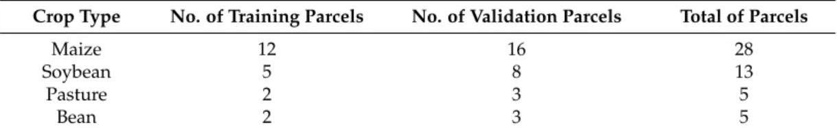
After selecting which band combination and classifier to use, images were added cumulatively to evaluate the improvement of the classification accuracies. Approximately 50% of the ground truth parcels identified in the field per crop were randomly chosen to train the classifiers, while the rest was used to validate the classification results (Table4). For the classification, only 4 crop classes were considered: maize, soybean, pasture and bean. Four other crop classes (sunflower, millet, cabbage and potato) were excluded due to their limited number of ground truth parcels.
Table 4.Ground truth parcels used to train the classifier and to validate the classification results.
Crop Type No. of Training Parcels No. of Validation Parcels Total of Parcels
Maize 12 16 28
Soybean 5 8 13
Pasture 2 3 5
Bean 2 3 5
2.3.3. Crop Irrigation Requirement Modelling
Crop irrigation requirements (CIRs) are defined as the total amount of water, expressed in water height (mm), applied to the crop throughout the entire irrigation season to fully satisfy the crop water requirements. CIRs were computed in this study according to the FAO 56 approach [13] using the IrrigRotation soil water balance simulation model [22].
The IrrigRotation (Figure4) model simulates the soil water balance for crop rotations, performing this simulation with a daily time step, and computesETc according to the dual crop coefficient
approach proposed by [13,14,35], as defined in Equation (3):
ETc“ pKsˆKcb`Keq ˆETo (3)
where ETc is the crop evapotranspiration (mm¨day´1), Kcb is the basal crop coefficient, Ke is the soil evaporation coefficient, Ks is the water stress coefficient and ETo is the reference crop evapotranspiration (mm¨day´1).Ksdescribes the effect of water stress on crop transpiration. For soil water-limiting conditions,Ks < 1, and when there is no soil water stress,Ks = 1. In this study, no water stress is assumed when simulating the soil water balance. TheKcb-NDVI retrieved from EO data providesKcbvalues adjusted to the field conditions, already incorporating water stress, in contrast to the standard tabulatedKcbvalues.
−
−
ETo is computed from meteorological data using the FAO Penman–Monteith (FAO-PM) method [13,14]. The required meteorological data variables include solar radiation (Rs) (MJ¨m´2¨day´1), maximum air temperature (Tmax) (˝C), minimum air temperature (Tmin) (˝C), maximum relative humidity (HRmax) (%), minimum relative humidity (RHmin) (%), average wind speed at a height of 2 m (u2) (m¨s´1)
and precipitation (mm¨day´1).
The estimation ofKerequires a daily water balance computation for the calculation of the soil water content remaining in the upper topsoil [13,14,35]. The soil water balance equation adopted in IrrigRotation model is defined as [36]:
∆R“`
P´ETc`Rg´Es`Ac´Dr˘∆t (4)
where∆Ris the variation of the volume of water stored in the root zone (mm),∆tis the time step
(day), Pis the precipitation (mm¨day´1), Rgis the irrigation (mm¨day´1),Acis the capillary rise (mm¨day´1),ETcis the crop evapotranspiration (mm¨day´1),Esis the runoff (mm¨day´1) andDris the drainage and deep percolation (mm¨day´1). In this model, the soil profile is divided into three different layers. In the top soil layer, soil evaporation occurs with plant transpiration. The second layer corresponds to the portion of the soil that is occupied by the roots and where water is only withdrawn by plant transpiration. The thickness of this layer increases during crop growth. The bottom layer lies between the crop root depthZr(t) on daytand the maximum root depth. The irrigation requirements are calculated based on the values of the available soil water (ASW) in the second layer and on the irrigation management options [22,37]. In the present study, an irrigation strategy of no water restrictions was evaluated.
2.3.4. Basal Crop Coefficient and Crop Growth Stage Estimation from EO Data
In this study, theKcbis determined empirically from theKcb-NDVI relationships applied within the Participatory multi-Level EO-assisted tools for Irrigation water management and Agricultural Decision-Support (PLEIADeS) project using Equation (5) [10,38]:
Kcb“1.5625ˆNDVI´0.1 (5)
where NDVI is the mean value of a crop type for each acquisition date. The NDVI time series are used to identify the lengths of crop growth stages (initial, crop development, mid-season and late-season) and the correspondingKcbcoefficients for the initial, mid-season and late-season periods (Figure5). This methodology in several studies has shown good agreement between the estimatedKcb-NDVI values and field measurements [10,21].Kcb-NDVI is a simplified version, as more physically-based
approaches to estimate the crop water requirements from EO data are available [39]. A previous study in the Lower Tagus Valley assessing the field applications for this methodology showed that it is suitable for operational irrigation management [40].
− −
− −
Δ Δ
− −
− − −
−
3. Results
3.1. NDVI and VV + VH Backscattering Time Series
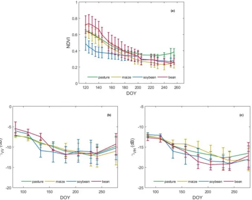
The time series of mean NDVI and VV + VH backscattering for the selected crop types are shown in Figure6. As observed in this figure, the average VV backscatter is higher than the average VH backscatter. The dynamic range of the VV backscatter is´12.31 dB to´5.49 dB, while the range of VH backscatter is´19.37 dB to´11.97 dB. NDVI values range from 0.23 to 0.73.
− −
− −
Figure 6.Mean NDVI (a) and gamma VV (b) and VH (c) backscattering time series for maize, soybean, pasture and bean.
Because the crop parameters were estimated from the NDVI and VV + VH time series, it can be seen in Figure6that the period covered by EO data corresponds to the second half of the growing season. The lack of data for the beginning of the growing season prevents the estimation of the seasonal crop irrigation requirements and its respective analysis. Due to this limitation, the focus of this study was only on crop water requirement estimation.
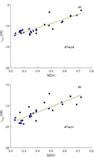
The behavior of the Sentinel-1A signal was also analyzed as a function of the NDVI. The backscattering coefficients were compared to the NDVI index calculated from SPOT-5 data with acquisition dates close to those of the Sentinel-1A acquisitions (Table5). Most of the image pairs used have a gap of only one to two days, yet for the pair Sentinel-1A 19 April and SPOT-5 30 April, there is a gap of 11 days. A square of the Pearson product-moment correlation coefficient (R2) of 79% was
γ
Figure 7.Scatterplots of the linear regression between the gamma VV + VH Sentinel-1A bands and the
NDVI band, (a,b), respectively.
Table 5.Image pairs used to compare optical and microwave observations.
Image/Month April May June July August
SPOT-5 30 15 4; 29 24 18; 28
Sentinel-1A 19 13 6; 30 24 17; 29
Based on this linear regression, two equations are proposed to compute theKcbvalues for epochs for which no optical images are available due to the existence of clouds. One equation uses the VV backscatter instead of the NDVI values (Equation (6)), while the other uses the VH backscatter values (Equation (7)):
KcbpVVq “0.116875ˆγVVpdBq `1.757031 (6) KcbpVHq “0.087813ˆγVHpdBq `1.984063 (7) whereγiis the gamma-calibrated backscattering coefficient in dB obtained from Equation (2) for each pixel of the SAR images.
Basal Crop Coefficient Estimation from EO Data
Table 6.Kcbvalues obtained from theKcb-NDVI approach.
Date DOY Maize Soybean Pasture Bean
30 April 120 0.9 0.7 0.9 1.0
5 May 125 0.9 0.6 0.9 1.0
10 May 130 0.8 0.6 0.9 1.0
15 May 135 0.8 0.5 0.8 1.0
20 May 140 0.8 0.5 0.8 0.9
25 May 145 0.7 0.5 0.7 0.8
4 June 155 0.6 0.5 0.7 0.7
9 June 160 0.6 0.5 0.6 0.7
14 June 165 0.5 0.5 0.6 0.6
19 June 170 0.5 0.5 0.6 0.6
24 June 175 0.5 0.4 0.5 0.5
29 June 180 0.4 0.4 0.5 0.5
7 July 185 0.4 0.4 0.5 0.5
9 July 190 0.4 0.4 0.5 0.5
14 July 195 0,4 0.4 0.5 0.4
19 July 200 0.4 0.4 0.5 0.4
24 July 205 0.3 0.3 0.4 0.4
8 August 220 0.3 0.4 0.4 0.4
13 August 225 0.3 0.4 0.4 0.3
18 August 230 0.3 0.3 0.4 0.3
28 August 240 0.3 0.3 0.5 0.3
7 September 250 0.3 0.3 0.5 0.3
12 September 255 0.3 0.4 0.5 0.3
3.2. Image Classification and Accuracy Assessment
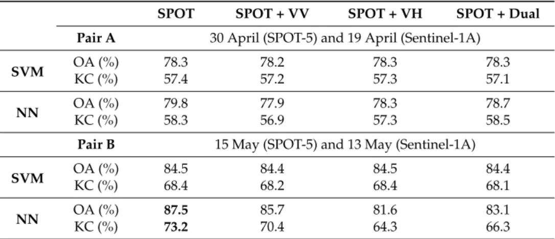
Analyzing the results of the SVM and NN classifiers for April and May 2015 using the four image combinations, the NN results exhibit, in general, a slight improvement compared to those from SVM (Table7). For these two acquisition dates (late season both for maize and soybean), the addition of the gamma backscattering bands did not increase the overall accuracy. The highest value obtained for the overall accuracy (87.5%) was obtained for the results of an NN classification using just the four spectral bands of the SPOT-5 image for 15 May.
Table 7. Overall accuracy (OA) and kappa coefficient (KC) values for the 4 data combinations for
2 acquisition dates.
SPOT SPOT + VV SPOT + VH SPOT + Dual
Pair A 30 April (SPOT-5) and 19 April (Sentinel-1A)
SVM OA (%)KC (%) 78.357.4 78.257.2 78.357.3 78.357.1
NN OA (%)KC (%) 79.858.3 77.956.9 78.357.3 78.758.5
Pair B 15 May (SPOT-5) and 13 May (Sentinel-1A)
SVM OA (%)KC (%) 84.568.4 84.468.2 84.568.4 84.468.1
NN OA (%)KC (%) 87.573.2 85.770.4 81.664.3 83.166.3
of the time series. No more images were added from late July, as the overall accuracies decreased and stabilized their values to approximately 85%.
Figure 8. Overall accuracies and kappa coefficients (%) obtained from the cumulative addition of SPOT-5 bands into the NN classification process.
The producer´s and user’s accuracies for the best multitemporal classification results are shown in Figure9. The producer’s accuracies were high for all crops, except for bean, while a low user’s accuracy was verified for pasture. According to Figure9and Table8, bean is slightly underestimated in the map as maize, whereas pasture is considerably overestimated in the map, mainly as maize, but also as soybean.
Figure 9.Individual class producer’s (PA) and user’s (UA) accuracies (%) for the best result from a
multitemporal classification of the SPOT-5 bands using the neural network classifier.
Table 8.Confusion matrix for the best result from a multitemporal classification of the SPOT-5 bands using the neural network classifier.
Ground Truth (pixels)
Crop Bean Maize Pasture Soybean Total
Bean 3580 309 85 15 3989
Maize 1027 71,145 68 1480 73,720
Pasture 23 2711 3643 227 6604
Soybean 4 3461 51 19,489 23,005
In Figure10is shown a detailed late-season map derived from the multitemporal classification of a SPOT-5 Take-5 time series using the NN classifier including images from 30 April to 4 June.
−
Figure 10.Extract of a map corresponding to the best result from a multitemporal classification of the
SPOT-5 bands using the neural network classifier.
3.3. Crop Water Requirement Modelling
TheEToandETcvalues for each crop type over the time series of this study are shown in Figure11.
−
Figure 11.Reference evapotranspiration (ETo) and crop evapotranspiration (ETc) for each crop (mm).
−
Figure 12.Total crop water requirement (m3¨day´1) volume.
Table 9.Total area of all of the parcels identified in the field for each crop type (ha).
Crop Type Total Area (ha)
Maize 1311.47
Soybean 302.87
Pasture 62.72
Bean 97.22
4. Discussion
In the NDVI time series in Figure6, the maize crop decreased from the end of mid-season until harvesting (senescence stage). This results from the fact that most of the maize parcels were sown in September/October 2014, while the first EO acquisition date was 26 March 2015 (DOY 85). The same trend was also observed in the VV + VH backscatter time series, indicating that both types of EO data are correlated. Although only half of a crop growth cycle is retrieved from the EO data, the results are promising because they demonstrate that this correlation is also possible for the late season period.
Bean parcels, sown in late February 2015, exhibited higher NDVI values in the beginning of the curve corresponding to the leaf development stage (Figure6). At the senescence stage, the bean crop presented the same trend as that of maize. Because soybean was sown in December 2014, the lower NDVI values in the beginning of the curve are explained by the crop growth stage (senescence) and by the typical short height of soybean (approximately 0.45 m). Pasture showed a smoother curve for the three time series, in agreement with the fact that pasture is always in the leaf development stage due to it being cut several times during the growing season.
In Figure7, a significant correlation is observed, especially between the VV backscatter and the NDVI values, demonstrating the consistency of both optical and microwave time series and that optical data affected by clouds can be replaced by microwave data. This overcomes one of the main limitations of these type of studies,i.e., the reduced amount of EO data due to meteorological conditions. This result agrees with those of [41], in which the potential of different TerraSAR-X incidence angles and polarizations for mapping sugarcane harvests, where a high correlation between the radar signal and NDVI index, calculated from SPOT-4/5, was observed. However, our results differ from those obtained during the AgriSAR campaign [42], in which gamma VH backscatter correlated strongly with NDVI for canola and field pea throughout the entire growth cycle. In AgriSAR, it was verified that among cereal crops, the correlation with NDVI is much weaker when analyzed over the entire growth cycle, exhibiting only a strong correlation for the initial vegetative growth stages until booting/inflorescence.
According to the overall accuracy and kappa coefficient values in Table7, the NN classification results were more accurate than those of the SVM classifier (~8% for the overall accuracy and ~15% for the kappa coefficient). SVM applied in [43] for land cover characterization using MODIS time series data was compared to two conventional non-parametric image classification algorithms: NN and classification and regression trees (CART). SVM generated an overall accuracy of 80% compared to 76% and 73% for NN and CART, respectively. However, some other studies reported that NN outperformed SVM and decision trees [44–46].
The addition of the gamma backscattering bands to the SPOT-5 optical bands did not reveal any improvement in the results of the SVM and NN classifications (Table7). In a previous study [47] of the Lower Tagus Valley, the use of a Sentinel-1A VH band together with the optical bands of a Landsat-8/OLI image enabled only a slight increase in the overall accuracy (1.6%) and in the kappa coefficient (2.5%) compared to the results of an SVM classification of the optical bands. Moreover, when adding only the Sentinel-1A VV band or both SAR bands to the optical bands, the overall accuracies and kappa coefficients were always lower than those obtained under the best band combination. Moreover, in [48], the addition of backscatter intensity derived from Radarsat-2 images to the surface reflectances derived from Landsat-8/OLI images for crop classification in Ukraine slightly improved the overall classification accuracy from 1.5% to 4.0%.
The use of multitemporal C-band Sentinel-1A images along with multitemporal SPOT-5 Take-5 images for crop classification in Wako-Kungo revealed an improvement of the overall classification accuracy when images are added cumulatively into the classification process. An overall accuracy of 91% (with a kappa coefficient of 81%) was obtained with a set of images from April 30 until June 4 (a total of 28 optical bands corresponding to the first 7 SPOT-5 Take-5 images of the time series), as expected, because they were acquired during and a few weeks after the field work when the crops were relatively vigorous. From that date on, classifications returned lower overall accuracies because there was a substantial decay in the NDVI and VV + VH backscatter values, indicating that the cultures are all in the last stage of senescence, having wilted and sometimes been already harvested.
In Table8, one can observe a significant misclassification between maize and pasture for the beginning of the time series, while a clear separation between soybean and bean seems to be evident, as expected from the analysis of Figure6. Pasture is the culture with the highest commission error (approximately 45%), meaning that the area occupied by this crop in the final map is significantly overestimated mainly due to misclassifications with maize, but also with soybean and bean. Bean has the highest omission error (approximately 23%), meaning that the area occupied by this crop in the final map is underestimated mainly due to misclassifications with maize.
and the off season. Hence, without a through characterization of the complete growing season and of the cultural and irrigation practices in the region, it is difficult to accurately estimate the irrigation water requirements. From the analysis of the calculated volumes (Figure12), it is possible to verify the decrease in the values over time, again due to the senescence stage shown by most crops.
Better classification results would have been obtained if EO data were available for the entire crop growing season; thus, it would have been possible to estimate the crop irrigation requirements for the Wako-Kungo irrigation perimeter.
5. Conclusions
The purpose of this study was to assess the potential of multitemporal and multisensor EO data (Sentinel-1A and SPOT-5 Take-5) for crop parameter retrieval and crop type classification for agricultural water management in Angola.
The integration of microwave data (Sentinel-1A) with optical data (SPOT-5 Take-5) did not reveal any improvement in land cover mapping. From the two supervised classification methods used, NN had the highest accuracy of approximately 88% (with a kappa coefficient of approximately 73%) compared to that of the SVM classifier (85% and 68% for the overall accuracy and kappa coefficient, respectively). Higher classification accuracies were expected when using SAR data; however, the unavailability of images for more than half of the crop cycle (only the end of mid-season until harvesting was available) did not permit a better discrimination among crops. A multitemporal NN classification using just the first seven SPOT-5 Take-5 images produced a late mid-season map with an overall accuracy of 91% (with a kappa index of 81%).
The improved temporal resolution of the SPOT-5 Take-5 images, used in this study to simulate the ESA Sentinel-2 time series, is relevant for a better identification of the different crop growth cycle stages that are often imperceptible when using more sporadic data. Higher temporal resolution time series allow the retrieval of realistic values forKcbinstead of the standard values proposed by FAO 56 [13] and, consequently, a better estimation of the crop’s irrigation requirements. However, this aspect was not fully exploited for the same reason mentioned previously,i.e., the lack of EO data for the complete growing season. Moreover, the consistency observed between the optical and microwave time series for all crop types enables the replacement of optical data affected by clouds with microwave data to increase the temporal resolution of the time series, providing a proxy measurement of crop development.
Acknowledgments:This study was developed in the scope of the ESA Alcantara initiative project (Ref: 14-P13) and the SPOT-5 Take-5 project (ID: 29142).
Author Contributions:Ana Navarro and João Rolim designed the study and did most of the writing. Irina Miguel
performed most of the pre-processing steps. João Catalão contributed to the results analysis and to the writing. Joel Silva, Marco Painho and Zoltán Vekerdy reviewed the paper.
Conflicts of Interest:The authors declare no conflict of interests.
References
1. Waldner, F.; Lambert, M.-J.; Li, W.; Weiss, M.; Demarez, V.; Morin, D.; Marais-Sicre, C.; Hagolle, O.; Baret, F.; Defourny, P. Land cover and crop type classification along the season based on biophysical variables retrieved from multi-sensor high-resolution time series.Remote Sens.2015,7, 10400–10424. [CrossRef]
2. Brisco, B.; Brown, R.J. Multi-date SAR/TM synergism for crop classification in Western Canada. Photogramm. Eng. Remote Sens.1995,61, 1009–1014.
3. Le Hegarat-Mascle, S.; Quesney, A.; Vidal-Madjar, D. Land cover discrimination from multitemporal ERS images and multispectral Landsat images: A study case in an agricultural area in France.Int. J. Remote Sens.
2000,21, 435–456. [CrossRef]
4. Ban, Y. Synergy of multitemporal ERS-1 SAR and Landsat TM data for classification of agricultural crops. Can. J. Remote Sens.2003,29, 518–526. [CrossRef]
6. Michael, J.H.; Ticehurst, C.J.; Lee, J.S.; Grunes, M.R.; Donald, G.E.; Henry, D. Integration of optical and radar classifications for mapping pasture type in Western Australia.IEEE Trans. Geosci. Remote Sens. 2005,43, 1665–1681.
7. McNairn, H.; Champagne, C.; Shang, J.; Holmstrom, D.; Reichert, G. Integration of optical and Synthetic Aperture Radar (SAR) imagery for delivering operational annual crop inventories.ISPRS J. Photogramm. Remote Sens.2009,64, 434–449. [CrossRef]
8. FAO. Use of remote sensing techniques in irrigation and drainage. In Proceedings of the Expert Consultation FAO-Cemagref, Montpellier, France, 2–4 November 1993; Food and Agriculture Organization United Nations: Rome, Italy, 1993.
9. Schultz, G.A.; Engman, E.T. Remote Sensing in Hydrology and Water Management; Springer-Verlag Inc.: New York, NY, USA, 2000.
10. D’Urso, G.; Richter, K.; Calera, A.; Osann, M.A.; Escadafal, R.; Garatuza-Pajan, J.; Hanich, L.; Perdigão, A.; Tapia, J.B.; Vuolo, F. Earth Observation products for operational irrigation management in the context of the PLEIADeSproject.Agric. Water Manag.2010,98, 271–282. [CrossRef]
11. Doorenbos, J.; Pruitt, W.O.Guidelines for Predicting Crop Water Requirements; FAO Irrigation and drainage paper No. 24; Food and Agriculture Organization of the United Nations: Rome, Italy, 1977; p. 179. 12. Pereira, L.S.; Allen, R.G. Crop water requirements. InCIGR Handbook of Agricultural Engineering: Land and
Water Engineering; Van Lier, H., Pereira, L.S., Steiner, F., Eds.; American Society of Agricultural Engineers: St. Joseph, MI, USA, 1999; Volume 1, pp. 213–262.
13. Allen, R.G.; Pereira, L.S.; Raes, D.; Smith, M.Crop Evapotranspiration: Guidelines for Computing Crop Water Requirements; FAO Irrigation and Drainage Paper No. 56; Food and Agriculture Organization of the United Nations: Rome, Italy, 1998.
14. Allen, R.G.; Wright, J.L.; Pruitt, W.O.; Pereira, L.S.; Jensen, M.E. Water requirements. InDesign and Operation of Farm Irrigation Systems, 2nd ed.; ASABE: St. Joseph, MI, USA, 2007; pp. 208–288.
15. Bastiaanssen, W.G.M.; Menenti, M.; Feddes, R.A.; Holtslag, A.A.M. Remote sensing surface energy balance algorithm for land (SEBAL): 1 Formulation.J. Hydrol.1998,212–213, 198–212. [CrossRef]
16. Allen, R.G.; Tasumi, M.; Morse, A.; Trezza, R.; Wright, J.L.; Bastiaanssen, W.; Kramber, W.; Lorite, I.; Robison, C.W. Satellite-based energy balance for mapping evapotranspiration with internalized calibration (METRIC)—Applications.J. Irrig. Drain. E2007,133, 395–406. [CrossRef]
17. Eldeiry, A.A.; Waskom, R.M.; Elhaddad, A. Using remote sensing to estimate evapotranspiration of irrigated crops under flood and sprinkler irrigation systems.Irrig. Drain.2016,65, 85–97. [CrossRef]
18. Neale, C.M.; Bausch, W.C.; Heerman, D.F. Development of reflectance-based crop coefficients for corn. Trans. ASAE1989,32, 1891–1899. [CrossRef]
19. Calera Belmonte, A.; Jochum, A.M.; Cuesta Garía, A.; Montoro Rodríguez, A.; LópezFuster, P. Irrigation management from space: Towards user-friendly products.Irrig. Drain. Syst.2005,19, 337–353. [CrossRef]
20. Osann Jochum, M.A.; Calera, A.; DEMETER partners. Operational space-assisted irrigation advisory services: Overview of and lessons learned from the project DEMETER. In Proceedings of the Earth Observation for Vegetation Monitoring and Water Management, Naples, Italy, 10–11 November 2005; D’Urso, G., Osann Jochum, M.A., Moreno, J., Eds.; American Institute of Physics: Melville, NY, USA, 2006; pp. 3–13.
21. Toureiro, C.; Serralheiro, R.; Shahidian, S.; Sousa, A. Irrigation management with remote sensing: Evaluating irrigation requirement for maize under Mediterranean climate condition.Agric. Water Manag.2016. [CrossRef]
22. Rolim, J.; Teixeira, J. IrrigRotation, a time continuous soil water balance model.WSEAS Trans. Environ. Dev.
2008,4, 577–587.
23. Diniz, A.C.Angola o Meio Físico e Potencialidades Agrárias; Instituto da Cooperação Portuguesa (ICP), Fundação Portugal-África: Lisbon, Portugal, 1998.
24. Diniz, A.C.; Aguiar, F.B.Zonagem Agro-Ecológica de Angola, 2nd ed.; Instituto da Cooperação Portuguesa (ICP), Fundação Portugal-África: Lisbon, Portugal, 1998.
25. Russo, A.T.; Oliveira, P.B.; Bisca, F.R. Reabilitação e modernização de aproveitamentos hidroagrícolas em Angola. A engenharia dos aproveitamentos hidroagrícolas: Actualidade e desafios futuros. In Proceedings of the Jornadas Técnicas APRH, LNEC, Lisbon, Portugal, 13–15 October 2011.
26. MDA (MacDonald, Dettwiler and Associates Ltd.).Sentinel-1 Product Definition; Ref: S1-RS-MDA-52-7440; MacDonald, Dettwiler and Associates Ltd.: Richmond, BC, Canada, 2011.
28. SASSCAL WeatherNet. Available online: http://www.sasscalweathernet.org/ (acessed on 2 December 2015). 29. Rouse, J.; Haas, R.; Schell, J.; Deering, D.; Harlan, J.Monitoring the Vernal Advancement of Retrogradation of
Natural Vegetation; Type III, Final Report; NASA/GSFC: Greenbelt, MD, USA, 1974.
30. Chang, C.-C.; Lin, C.-J. LIBSVM: A Library for Support Vector Machines. Available online: http://www.csie. ntu.edu.tw/~{}cjlin/papers/libsvm.pdf (accessed on 25 May 2016).
31. Wu, T.-F.; Lin, C.-J.; Weng, R.C. Probability estimates for multi-class classification by pairwise coupling. J. Mach. Learn. Res.2004,5, 975–1005.
32. Hsu, C.-W.; Chang, C.-C.; Lin., C.-J.A Practical Guide to Support Vector Classification; National Taiwan University: Taipei, Taiwan, 2010.
33. Rumelhart, D.; Hinton, G.E.; Williams, R.J. Learning internal representation by error propagation. InParallel Distributed Processing; MIT Press: Cambridge, MA, USA, 1987; Volume 1, pp. 318–362.
34. Richards, J.A.Remote Sensing Digital Image Analysis; Springer-Verlag: Berlin, Germany, 1999.
35. Teixeira, J.L.; Fernando, R.M.; Pereira, L.S. RELREG: A model for real time irrigation scheduling. InCrop-Water-Simulation Models in Practice; Pereira, L.S., van den Broek, B.J., Kabat, P., Allen, R.G., Eds.; WageningenPers: Wageningen, The Netherlands, 1995; pp. 3–15.
36. Rolim, J.; Catalão, J.; Teixeira, J.L. The influence of different methods of interpolating spatial meteorological data on calculated irrigation requirements.Appl. Eng. Agric.2011,27, 979–989. [CrossRef]
37. Allen, R.G.; Pereira, L.S.; Smith, M.; Raes, D.; Wright, J.L. FAO-56 dual crop coefficient method for estimating evaporation from soil and application extensions.J. Irrig. Drain. E2005,131, 2–13. [CrossRef]
38. D’Urso, G.; Calera Belmonte, A. Operative approaches to determinecrop water requirements from Earth Observation data: Methodologies and applications. In Proceedings of the Earth Observation for Vegetation Monitoring and Watermanagement, Naples, Italy, 10–11 November 2005; D’Urso, G., OsannJochum, M.A., Moreno, J., Eds.; American Institute of Physics: Melville, NY, USA, 2006; pp. 14–25.
39. Vuolo, F.; D’Urso, G.; de Michele, C.; Bianchi, B.; Cutting, M. Satellite-based irrigation advisory services: A common tool for different experiences from Europe to Australia.Agric. Water Manag.2015,147, 82–95.
[CrossRef]
40. Vilar, P.; Navarro, A.; Rolim, J. Utilização de imagens de deteção remota para monitorização das culturas e estimação das necessidades de rega. In Proceedings of the VIII Conferência de Cartografia e Geodesia, Ordem dos Engenheiros, Lisbon, Portugal, 29–30 October 2015.
41. Baghdadi, N.; Cresson, R.; Todoroff, P.; Moinet, S. Multitemporal observations of sugarcane by TerraSAR-X images.Sensors2010,10, 8899–8919. [CrossRef] [PubMed]
42. MDA (MacDonald, Dettwiler and Associates Ltd.).AgriSAR2009: Final Report—Vol. 1 Executive Summary; Ref: RX-RP-53-1382-001; MacDonald, Dettwiler and Associates Ltd.: Richmond, BC, Canada, 2011. 43. Shao, Y.; Lunetta, R.S. Comparison of support vector machine, neural network, and CART algorithms for
the land-cover classification using limited training data points.ISPRS J. Photogramm. Remote Sens.2012,70,
78–87. [CrossRef]
44. Du, P.; Xia, J.; Zhang, W.; Tan, K.; Liu, Y.; Liu, S. Multiple classifier system for remote sensing image classification: A review.Sensors2012,12, 4764–4792. [CrossRef] [PubMed]
45. Gallego, J.; Kravchenko, A.; Kussul, N.; Skakun, S.; Shelestov, A.; Grypych, Y. Efficiency assessment of different approaches to crop classification based on satellite and ground observations. J. Autom. Inf. Sci.
2012,44, 67–80. [CrossRef]
46. Gallego, F.J.; Kussul, N.; Skakun, S.; Kravchenko, O.; Shelestov, A.; Kussul, O. Efficiency assessment of using satellite data for crop area estimation in Ukraine.Int. J. Appl. Earth Observ. Geoinf.2014,29, 22–30. [CrossRef] 47. Saraiva, C.; Navarro, A. Avaliação do potencial das imagens Sentinel-1 para identificação de culturas agrícolas. In Proceedings of the VIII Conferência de Cartografia e Geodesia, Ordem dos Engenheiros, Lisbon, Portugal, 29–30 October 2015.
48. Skakun, S.; Kussul, N.; Shelestov, A.Y.; Lavreniuk, M.; Kussul, O. Efficiency assessment of multitemporal C-band Radarsat-2 intensity and Landsat-8 surface reflectance satellite imagery for crop classification in Ukraine.IEEE J. Sel. Top. Appl.2015. [CrossRef]
![Figure 5. Basal crop coefficient (K cb ) curve (adapted from [13]).](https://thumb-eu.123doks.com/thumbv2/123dok_br/15755299.638747/10.892.263.633.913.1124/figure-basal-crop-coefficient-k-cb-curve-adapted.webp)