Inverse Modelling for Estimation of Average
Grain Size and Material Constants
- An Optimization Approach
P. Kathirgamanathan and T. Neitzert
∗Abstract—The goal is to build up an inverse model capable of finding the average grain size history dur-ing an extrusion process and other material constants by using simulated strain and temperature values. This problem of finding the parameter values is based on linear and nonlinear least-squares regressions, cou-pled with microstructure control models and the so-lution of a finite element extrusion model. The prob-lem is ill posed and we use the Tikhonov’s regulari-sation to stabilise the solution process. Further some of the parameters in the model are linear and some are nonlinear. We determine the linear parameters using simple linear algebra and for the computation of non-linear parameters we use
M
ATLAB’s routine lsqnonlin.Keywords: Extrusion; Inverse problem; Parameter es-timation; Optimization.
1
Introduction
Numerical modelling of extrusion may be used during a design process to assess the extruded material proper-ties. The extrusion simulation describes the material flow through the die. An extrusion model, which is capable of describing the behaviour of material flow, requires the following input data: (a) material data such as Young’s modulus, coefficient of expansion, Poisson’s ratio, inelas-tic heat fraction, specific heat, density, conductivity, flow stress-strain relationship, (b) die design variables and (c) process variables such as ram speed, initial temperature and friction factors.
In reality, material data can be measured using available measuring instruments, but the optimal values of die de-sign variables and process variables are often unknown. In a previous paper[3], we formulated a non-linear least squares inverse model in which the optimal values of die design variables and process variables were estimated to achieve a certain grain size. In the approach the following
∗Manuscript received March 01, 2008. This work was supported
by Technology New Zealand; Authors are with School of Engineer-ing, Auckland University of Technology, Auckland, New Zealand; email: [email protected], [email protected]
average grain size equation [7],[8]
d=α
dε dtexp
Q RT
β
(1)
was used as optimizing criteria to terminate the problem.
In equation (1),Qis an activation energy,dis the average
recrystallized grain size, T is the temperature, dε
dt is the
strain rate andR is the universal gas constant.
The values of constants α and β are based on
experi-mental observations and therefore the uncertainty of the constants is very high. Small changes in these values can cause variation in the grain size estimation. The success-ful application of equation (1) depends on the accuracy of the parameters. Methods to identify the optimal values
ofαandβ are therefore an important part of modelling
extrusion processes to increase the reliability of the nu-merical simulation.
In the present work an alternative method is proposed. The idea is to develop an inverse model for estimat-ing grain size history, usestimat-ing inverse modellestimat-ing techniques available in the literature. Inverse modelling avoids the
use of αand β for the grain size history estimation. To
do so we consider the problem in which the material properties of the billet as well as process and die design
parameters are known but the material constants α, β
and grain size d are not known. The accuracy of the
model is examined by using simulated temperature and strain data (generated by the forward model) to which normally-distributed relative noise has been added. We design the inverse model as a least squares minimisation problem associated with an ABAQUS finite element solu-tion of an extrusion process. This is an ill-posed problem and we solve it using regularisation methods.
2
Forward Problem
The thermo-mechanical behaviour of the extrusion pro-cess can be described mathematically using conservation of mass, momentum and energy as follows [4], [5], [6]: The mass conservation is
Dρ
whereρis the density of the material andVis the velocity vector.
The momentum conservation is
ρDV
Dt =∇ ·σ+ρf (3)
wheref is the body force per unit mass, andσis Cauchy
stress tensor.
The energy conservation is
ρc
∂T
∂t +V· ∇T
=−∇ ·(−k· ∇T) + ˙Q (4)
whereT is the temperature,cis the specific heat,k=kI,
kdenotes thermal conductivity,Tis the temperature and
˙
Qis the rate of heat generated per unit volume.
Equations (2),(3) and (4) can be solved using finite ele-ment methods. We have impleele-mented a solution proce-dure using ABAQUS to obtain temperature and strain histories during the deformation process. Once the tem-perature and strain values are obtained, the average grain size at a nodal point can be calculated using equation (1).
3
Inverse Problem
The goal of inverse modelling is the extraction of model parameter information from data. It is a subject, which supplies tools for the proficient use of data in the estima-tion of constants appearing in the models. In this inverse problem, the structure of the equation is known; outputs,
temperature (T) and strain (ε) values are available.
Av-erage grain size history and parametersαandβ are the
unknowns.
In this section a model is formulated to obtain the best or
optimal estimate of grain size history,αandβ appearing
in equation (1) from temperature and strain estimations made at some nodes in the material inside the forming zone. The microstructural model given equation (1) can be rewritten to solve for strain rate as follows.
dε dt =
d α
1/β
exp
−Q RT
(5)
Therefore the strain is
ε(t) =
Z t
0
d(τ)
α 1/β
exp
− Q RT(τ)
dτ
=
Z t
0
K(t, τ)D(τ)dτ (6)
where the kernelK(t, τ) is:
K(t, τ) = exp
−Q RT(τ)
(7)
and
D(τ) =
d(τ)
α β1
(8)
If n temperature and strain values are available at the
node (X1, Y1, Z1) between 0 andtf and suppose that we
wish to determine D(τ) at times τ0 = 0, . . ., tf, then
discretising (6) by the trapezoidal rule gives a system of linear equations
e= A(p)q (9)
where e = [ε(0), . . . , ε(tf)] T
, Aij = K(ti, τj)βij, q = [D(τ0), . . . , D(τf)]T and p = [Q], and βij is a quadra-ture weight. Generally, minimising an objective
func-tion solves inverse problems. The objective funcfunc-tion Z
that provides minimum variance estimates is the ordi-nary least squares function
minimize Z(p, q) =kA(p)q−ek2
2 (10)
If the value of activation energy Q is known then the
problem becomes a linear least square problem and can be solved easily. But the coefficient matrix of problem (10) always has a very large condition number and is ill posed. Therefore well posedness must be restored by restricting the class of admissible solutions. This can be achieved using regularisation methods [1]. With Tikhonov’s regu-larisation, we introduce the regularised objective function
Z(q) = kAq−ek2
2+λ
2
kLqk2
2 (11)
where kAq−ek2
2 is the residual norm (or data misfit
function), and kLqk2
2 is the solution norm. We will be
interested in the minimisation of the function Z(q) for
different values ofλ. Note that the objective functionZ
is the 2-norm of the following system of equations
A λL
q=
e 0
,
whereLis the regularisation operator and λis the
regu-larisation parameter.
If the value ofQis not known then the problem becomes
a nonlinear least square problem as follows.
Z(q, p) =kA(p)q−ek2
2+λ
2
kLqk2
2. (12)
Since the equation (12) has a combination of linear
pa-rameters q and non-linear parameters p, we separate
the solution process into two steps. We find the
non-linear parameter p by constructing an iterative
proce-dure, where at each iteration a linear sub-problem is
solved to estimate the linear parameter qcorresponding
to that particular value ofp.
Now taking natural logarithms of both sides of the equa-tion (8) and rearranging gives
ln(D) =mln(d) +C (13)
wherem= 1
β andC=
1
β ln 1
α
. Now supposen+ 1D
values are available and we wish to determine the
corre-spondingdvalues. This gives
A
B C
Figure 1: Three considered nodes on deformed mesh
where
K=
m 0 . . . 0 0 0 m . . . 0 0
..
. ... ... ... ...
0 0 . . . m 0 0 0 . . . 0 m
y=
lnd1 d0
lnd2 d0
.. . lndn−1
d0
lndn
d0
, f =
lnD1 D0
lnD2 D0
.. . lnDn−1
D0
lnDn
D0
Now the minimisation problem for estimatingyis
formu-lated as
min
y kKy−fk
2
2. (15)
It is a linear problem and therefore the grain size history
d1, d2, . . . , dncan be calculated with reasonable accuracy provided the initial grain size is known.
4
Applications
In this section, we present numerical simulations to demonstrate the solution process and evaluate the
ac-curacy of the model. To do so, we consider an
in-put of temperature and strain values data generated at three elements A, B, C as shown in Figure 1 from a FE-simulation of extrusion using ABAQUS. The data
values used in the simulation of extrusion are:
ini-tial temperature of work piece and die respectively are
T = 500oC and T = 450oC, work piece’s Young’s
modulus E = 7 ×10¹⁰
P a, coefficient of expansion
8.4×10⁻⁵ oC−1 at T = 20 oC, Poisson’s ratio 0.35,
A
10−2
1013.8
1013.9
residual norm || A q − e ||2
solution norm || q ||
2
B
Total Error
Misfit Error Error due to
regularization
Optimal λ
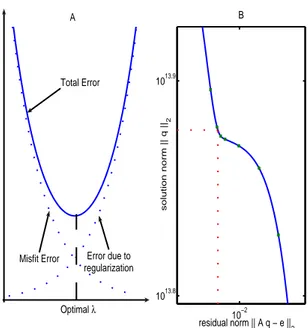
Figure 2: (A):Total error, (B) L-curve.
inelastic heat fraction 0.9, specific heat 910J kg−1K−1,
density= 2750 kgm−3, conductivity 204 W m−1K−1
when T = 0 oC, 225 W m−1K−1 when T = 300 oC,
die material’s Young’s modulus E = 20×1010
P a,
co-efficient of expansion 8.4×10⁻⁵ oC−1 at T = 20 oC,
Poisson’s ratio 0.30, inelastic heat fraction 0.9, specific
heat 450 J kg−1K−1, density 7200 kgm−3, conductivity
204 W m−1K−1 when T = 0 oC, 225 W m−1K−1 when
T = 300oC.
4.1
Estimation of
d
(
t
)
for known value of
ac-tivation energy
Q
If the value ofQis known, we will have to solve equation
(11) to estimate the grain size. The minimization
problem given by equation (11) depends on the optimal
value of the regularization parameter λ. A number
of techniques have been discussed in the literature[2] for estimating an optimal value of a regularization
parameter. Here we use the L-curve criteria to
esti-mate the parameter values. It is based on minimizing the total error equation (11) as shown in Figure 2.
A good regularization parameter λ should provide a
fair balance between data misfit error and
regulariza-tion error. The L-curve method shown in figure 2B
is based on minimizing total error as shown in Figure 2A.
Once the optimal value of λ is known, we estimate
q = [D(τ0), . . . , D(τf)]
T
easily and then using equation
(15) valuesy=hD1
D0, . . . , Dn
D0
iT
are calculated. Figure 3 shows the graph of equation (13) for the initial grain size
4.7 4.8 4.9 5 5.1 5.2 5.3 5.4 0
5 10 15 20 25
ln d
ln D
Final Value (lowest value)
Figure 3: Graph of Equation (13)
The accuracy of value Q we use in equation (1) may or
may not be very high since it is based on experimental
observations and the accuracy of estimation of dis also
subject to error. Therefore it is appropriate to analyze
the effect of inaccuracy of the Q value. To investigate
we changed the Q values, while all other values are
un-changed. Table (1) shows the optimal values of α and
β for the respective values ofQ obtained using the
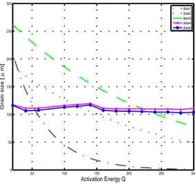
pro-posed method. Figure 4 depict the comparison of grain size variation. Data 4 in this graph is the grain size esti-mation using the proposed method and data 5 is the grain size variation obtained by equation (1)for the respective
α and β values given in table (1). Data 1, Data 2 and
Data 3 respectively are the grain size values for (α= 278
&β=−0.080), (α= 200 &β=−0.020) and (α= 279 &
β =−0.018) by equation (1). WhenQis underestimated,
the average grain size estimated value using equation (1) is higher than it used to be and increases approximately
quadratically with decreasing Qvalue. WhenQ is
over-estimated, the average grain size estimated value is lower than it used to be and decreases approximately
quadrat-ically with increasing Qvalue. The graph of Data 4 and
Data 5 are approximately the same. This shows that
even if the Qvalue is wrong, it is possible to estimated
accurately using equation (1) if appropriateαandβ
val-ues are available. It is not achievable in a real practical environment, but can be only possible through inverse modelling techniques.
4.2
Estimation of
d
(
t
)
for unknown value of
activation energy
Q
Here the problem is concerned with the estimation of
grain sized(t) values and the activation energy (Q). This
estimation process contains a combination of a nonlinear
parameter (Q) and linear parameters (d(t)). This is
dif-50 100 150 200 250 300
0 50 100 150 200 250 300
Activation Energy Q
Grain size [
µ
m]
data1 data2 data3 data4 data5
Figure 4: Grain size vs Q for different material constants
Q β α
20 -0.044 140
50 -0.080 278
100 -0.026 209
140 -0.020 200
180 -0.019 240
220 -0.018 279
300 -0.019 412
Table 1: % of variation with Q values
ferent from a linear problem and therefore we cannot only use linear algebra to solve this problem. This problem can be solved by constructing an iterative procedure as mentioned above. Alternatively we can solve the
equa-tion (12) for a sequence ofQvalues to get a best value for
Q which minimizes equation (12), since we have only one nonlinear parameter. Figure 5A, 5B respectively shows the variation of Z with Q at the nodes A, B, C for the
ram speed 12.5 mm s−1 and 6.5 mm s−1. The graphs
clearly show that the best value of Qis not same for all
cases. In the literature we can find that the activation energy of the material varies with temperature. During the extrusion process the temperature inside the defor-mation zone is not constant everywhere. Therefore using
constant Q value in equation (1) will not give an
accu-rate result unless appropriate values ofαandβare used.
Again the estimation ofαandβ which suits theQvalue
is not achievable in a real practical environment.
5
Summary and conclusion
20 40 60 80 100 120 140 0.1
0.2 0.3 0.4 0.5 0.6 0.7 0.8 0.9
Activation Energy Q
Objective Function Z
A
20 40 60 80 100 120 140
0.2 0.25 0.3 0.35 0.4 0.45 0.5 0.55
Activation Energy Q
Objective Function Z
B
data1 data2 data3
data1 data2 data3
Figure 5: Z vs Q
other material constants appearing in the model. The approach is based on a non-linear least squares estima-tion using simulated temperature and strain value his-tory inside the deformation zone. Since the problem is ill-posed we apply Tikhonov’s regularisation method to stabilise the solution process. Some of the parameters in the problem are linear and some are nonlinear. We determined the linear parameters using simple linear al-gebra and for the computation of non-linear parameters
we used
M
ATLAB’s routinelsqnonlin. The optimal valueof the regularisation parameter is obtained using the lin-ear L-curve for the linlin-ear problem.
Firstly, the usefulness of an inverse modeling technique in the grain size estimation process has been demon-strated. The inverse modelling technique has been
ap-plied to equation (1) with the situation in whichα,βand
Qvalues are unknown. Secondly, it has been shown that
the error in traditional destimation increases
quadrati-cally with the error in Q if the α and β values are
ad-justed accordingly to cater forQ. The appropriate values
ofαandβ can only be found using the above mentioned
inverse modelling technique. Thirdly, it has been demon-strated the optimal value of the activation energy inside the deformation region is not constant and varies with
the temperature. Therefore the traditional destimation
using equation (1) with constant values of Q, α and β
will not give the accurate value if the temperature inside the deformation zone is not constant.
References
[1] Hansen C. P, Rank-deficient and discrete ill-posed
problems, SIAM, Philadelphia, PA, 1997.
[2] Hansen C. P., Regularization tools: A MATLAB
package for analysis and solution of discrete ill-posed
problems, Danish Computing Center for Research and Education, 1993.
[3] Kathirgamanathan P., Neitzert T., “Optimal pro-cess control parameters estimation in aluminium
ex-trusion for given product characteristics,”Submitted
to The International Conference of Mechanical En-gineering, 2008.
[4] Lee G., Kwak D., Kim S., Im Y., “Analysis and
de-sign of flat-die hot extrusion process,”International
Journal of Mechanical Sciences, V44, pp.915–934, 2002
[5] Reddy V. R., Sethuraman R., Lal G. K., “Upper-bound and finite-element analysis of
axisymmet-ric hot extrusion,” Journal of Materials Processing
Technology, V57, pp.14–22, 1996
[6] Storen S., “The theory of extrusion- Advances and
challanges,”Int. J. Mech. Sci, V35, N12, pp. 1007–
1020, 1993
[7] Venugopal S., Rodriguez P., “Strategy for the de-sign of thermomechanical processes for AISI type 304L stainless steel using dynamic materials model stability criteria and model for the evolution of
mi-crostructure,” Journal of Materials Science, V39,
pp. 5557–5560, 2004
[8] Venugopal S., Medina E. A., Malas I., Medeiros S., Frazier W. G., “Optimization of microstructure during deformation processing using control theory
principles,” Scripta materialia, V36, pp. 347–353,