J. of the Braz. Soc. of Mech. Sci. & Eng. Copyright 2012 by ABCM April-June 2012, Vol. XXXIV, No. 2 / 105
Liércio A. Isoldi
[email protected] Universidade Federal do Rio Grande Escola de Engenharia 96021-900 Rio Grande, RS, Brazil
Cristiano P. Oliveira
[email protected] Universidade Federal do Rio Grande Programa de Pós-Graduação em Modelagem Computacional – PPGMC 96021-900 Rio Grande, RS, BrazilLuiz A. O. Rocha
[email protected] Universidade Federal do Rio Grande do Sul Departamento de Engenharia Mecânica 90050-170 Porto Alegre, RS, BrazilJeferson A. Souza
[email protected] Universidade Federal do Rio Grande Escola de Engenharia 96021-900 Rio Grande, RS, BrazilSandro C. Amico
[email protected] Universidade Federal do Rio Grande do Sul Departamento de Engenharia de Materiais 91501-970 Porto Alegre, RS, BrazilThree-Dimensional Numerical
Modeling of RTM and LRTM
Processes
Resin Transfer Molding (RTM) is a manufacturing process in which a liquid resin is injected into a closed mold pre-loaded with a porous fibrous preform, producing complex composite parts with good surface finishing. Resin flow is a critical step in the process. In this work, the numerical study of the resin flow in RTM applications was performed employing a general Computational Fluid Dynamics software which does not have a specific RTM module, making it necessary to use the Volume of Fluid method for the filling problem solution. Examples were presented and compared with analytical, experimental and numerical results showing the validity and effectiveness of the present study, with maximum difference among these solutions of around 8%. Besides, based on the computational model for the RTM process, a new computational methodology was developed to simulate Light Resin Transfer Molding (LRTM). In this process, resin is injected into the mold through an empty injection channel (without porous medium) which runs all around the perimeter of the mold. The ability of FLUENT package to simulate geometries which combine porous media regions with open (empty) regions was used. Two specific cases were simulated, showing the differences in time and behavior between RTM and LRTM processes.
Keywords: Resin Transfer Molding (RTM), Light Resin Transfer Molding (LRTM), resin flow, computational modeling, FLUENT® software
Introduction1
The use of composite materials has increased worldwide since the 50s as an alternative to heavy metals and other traditional materials. Many different industrial techniques have been developed for the manufacturing of composite materials. Among them, Liquid Composite Molding (LCM) techniques, such as Resin Transfer Molding (RTM), are considered attractive processes for fabricating low-to-medium volume composite parts of various sizes. In addition, RTM offers the versatility to produce parts of complex shapes and features. The process consists of two main steps. The mold filling step involves injecting a thermoset resin mixed with catalyst and/or initiators into a net-shaped mold cavity containing a dry fibrous unit, called the preform. The formulated resin permeates through the porous network formed by the fibers, yielding a saturated preform. In the second step, the mixture is usually subjected to heating that hardens the resin around the fibers, and produces the composite part (Nielsen and Pitchumani, 2002). The mold filling step is a critical aspect of the RTM process, being the focus of this work.
At present, most of the difficulties associated with RTM revolve around the filling stage. In order to create an acceptable composite part, the preform must be completely impregnated with resin. This is largely controlled by the fluid dynamics of the resin flow into the fiber reinforcement. The numerical simulation of the mold filling is important in assisting the design of RTM molds. Obviously, it is more economically viable to run numerical simulations before constructing the mold than to modify an existing mold. Besides, it minimizes the risk of producing defective parts.
Paper received 25 February 2011. Paper accepted 4 December 2011 Technical Editor: Francisco Cunha
The most used approach for modeling resin transport within a porous medium is to consider that the fluid flow can be determined by the Darcy’s Law, which associates the velocity of the fluid with the pressure drop inside the porous medium. The pressure field is obtained by combining the mass conservation equation and the proposed Darcy's equation, resulting in a single differential equation for the pressure (Souza, Rocha and Amico, 2007). There are many methods used to solve the second order differential equation developed for the pressure, but only a few simple cases, with specific fluid flow and geometry characteristics, have a closed (analytical) solution. Therefore, a numerical technique is commonly used to solve this equation (Ballata, Walsh and Advani, 1999; Modi, Simacek and Advani, 2003). Several numerical approaches are available for the pressure field determination, and the most frequently used formulations are based on finite differences, finite elements or finite volumes.
Nowadays, the most used techniques for the numerical simulation of RTM are: the Finite Element/Control Volume (FE-CV) and the Volume of Fluid (VOF) methods. For the RTM flow front line advancement determination in a single fluid model with the FE-CV method, the FAN technique is normally used (Bruschke and Advani, 1990; Souza et al., 2008). The VOF method is usually applied to track the flow front interface between resin and air in two phases RTM models (Shojaei, Ghaffarian and Karimian, 2004; Yang et al., 2008).
is injected into the mold through an injection channel and runs all around the perimeter of the mold through an empty channel (without porous medium). LRTM is a variation of the conventional RTM process, where vacuum is used to drive resin flow through the fibrous reinforcement within a closed mold. In this low pressure (below 1 bar) infiltration, resin is injected peripherally in the mold, converging to a central gate. The numerical solution of LRTM has practical engineering interest, e.g. in the definition of the central gate position, and has not been sufficiently reported by the scientific community.
Therefore, in the present work, a procedure for the numerical simulation of the mold filling in the RTM process is presented. This procedure is based on the VOF method and uses the FLUENT® commercial code. A few case studies are solved to allow comparison of analytical, experimental and numerical (with PAM-RTM® software) results in order to validate and show the potential use of the present computational modeling to solve 2D and 3D RTM problems. In addition, based on the previous model, a new computational methodology was developed for the numerical simulation of the LRTM process. This methodology explores the ability of FLUENT® software to analyze geometries which combine porous media with open (empty) regions.
Nomenclature
F = external force, N f = resin volume fraction
g = gravitational acceleration, m/s² i = representing the x, y and z directions j = representing the x, y and z directions K = permeability, m²
P = pressure, Pa
r = flow front radial position, m r0 = injection port radius, m t = time, s
V = velocity, m/s
f
x = resin front line position, m
Greek Symbols ε = porosity µ = viscosity, Pa.s ρ = density, kg/m³ τ = stress, Pa
∇ = gradient operator
Mathematical Modeling
In the RTM process, resin flows through a fibrous reinforcement which can be modeled as a porous medium. Hence, this flow can be assumed to follow the Darcy’s Law, which states that the flow rate of resin per unit area is proportional to the pressure gradient and inversely proportional to the viscosity of the resin (Bejan, 2004; Morren et al., 2009). The mathematical formulation for this phenomenon is given by:
ij i
K
V P
µ
= − ∇ , (1)
where Vi is the velocity vector , µ is the viscosity of the resin, Kij
is the permeability tensor of the fiber reinforcement, ∇ is the gradient operator, P is the pressure and the indexes ,i j=1, 2, 3 represent the ,x y and z directions, respectively. Considering the
resin with constant physical properties and as an incompressible fluid, the mass conservation can be stated as:
0
i V
∇ ⋅ = . (2)
The Volume of Fluid (VOF) Method
In the VOF method, the momentum, continuity and volume fraction transport equations must be solved simultaneously. In this work, the VOF solution is obtained with the FLUENT® software – a general CFD (Computational Fluid Dynamic) package based on the Finite Volume Method (FVM) which includes a VOF module for the solution of problems with two or more immiscible fluids where the position of the interface between the fluids is of interest (FLUENT, 2008). A single set of momentum equations is applied to all fluids, and the volume fraction of each fluid in every computational cell is tracked throughout the domain (Silva et al., 2008).
For the RTM simulation, the two phases involved in the problem are the resin (liquid phase) and the air (gaseous phase). Thus, the model is composed of the continuity equation, given by:
( )
Vi 0t
ρ ρ
∂ +∇⋅ =
∂ ; (3)
the equation for the resin volume fraction f , defined by:
( )
( )
0i f fV t ∂ + ∇ ⋅ =
∂ ; (4)
and the momentum equation, given by:
( )
i(
)
i i ij i i
V
V V P g F
t ρ
ρ µτ ρ
∂
+ ∇ ⋅ = −∇ + ∇ ⋅ + +
∂ , (5)
being ρ the density, t the time, τij the stress tensor, gi the
gravitational acceleration vector and Fi an external force vector.
In FLUENT®, porous media are modeled by adding a source term to the standard momentum equations such as (FLUENT, 2008):
i i
ij
F V
K µ
= − . (6)
Combining Eq. (5) and Eq. (6) and considering that Fi is very
large because Kij is very small (~ 1 10× −10), it is possible to
simplify Eq. (5) as follows:
i ij
P V
K µ
∇ = − . (7)
It is important to emphasize that Eq. (7) represents the Darcy’s Law as well as Eq. (1).
Validation of the Proposed Model
J. of the Braz. Soc. of Mech. Sci. & Eng. Copyright 2012 by ABCM April-June 2012, Vol. XXXIV, No. 2 / 107 commercial code for the numerical simulation of RTM problems,
being based on Darcy’s Law and on the Finite Element Method (FEM) (PAM-RTM, 2008). In addition, a three-dimensional RTM problem is analyzed. A mold with an inlet region without porous medium is used. A numerical simulation is carried out disregarding the inlet nozzle and the results are compared with those obtained with PAM-RTM® software. Then, another simulation considering the inlet nozzle is made, comparing this study with experimental results.
Rectilinear Flow
In this case, the resin is boundary injected from the left side of a rectangular mold (Fig. 1). Reinforcement with isotropic permeability
10 2 3.00 10
K= × − m and porosity ε =0.70 was studied. Then, a resin
(density ρ =920.00kg m/ 3 and viscosityµ=0.06Pa s⋅ ) is injected into the rectangular cavity of the mold under a constant injection pressure P0=0.35 10× 5Pa. This problem can be considered one-dimensional since the resin front line is moving in a straight line normal to the bottom and top mold walls (Silva et al., 2008). The computational domain was discretized using an unstructured mesh with triangular cells.
Figure 1. Computational domain for the rectilinear flow.
For constant injection pressure, the flow front solution can be obtained analytically as follows (Hattabi, Echaabi and Bensalah, 2008):
0 2
f
KP t x
µε
= , (8)
being xf the resin front line position and t the injection time.
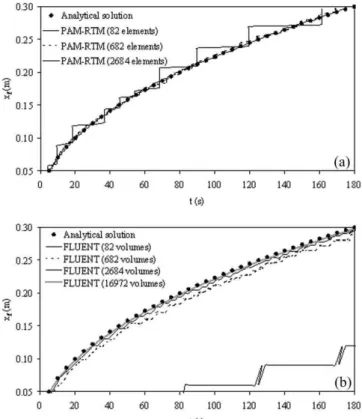
Figure 2 presents the comparison between the flow front position obtained with the analytical solution and the numerical solution generated by PAM-RTM® and FLUENT®. Analyzing Fig. 2, it can be seen that both numerical formulations were able to adequately determine the flow front position as a function of time. However, the FLUENT® solution (VOF method) seems to be more sensitive to grid refinement than that of the PAM-RTM®.
Radial Flow
The second test problem is schematically shown in Fig. 3. This is a two-dimensional problem where the resin flow advances at the same velocity in all directions. The resin injection is obtained by applying a prescribed pressure P0 at the center of the geometry. The resin and reinforcement properties and the injection pressure are the same used in the rectilinear flow simulation.
Figure 2. Rectilinear flow solution: (a) Analytical × PAM-RTM® and (b) Analytical × FLUENT®.
Figure 3. Computational domain for the radial flow.
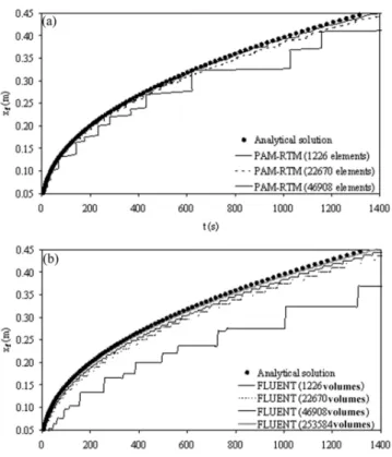
The problem was discretized using an unstructured mesh with triangular cells. In Fig. 4, the results obtained with FLUENT® and PAM-RTM® are compared with the analytical solution given by (Rudd, 2005):
(
)
2 2 2
0
0 0
1 ln
2 2
r
t r r r
KP r
µε
= − −
, (9)
Figure 4. Radial flow solution: (a) Analytical × PAM-RTM®
and (b) Analytical × FLUENT®.
Again, both numerical solutions followed well the analytical solution. Here again, higher grid refinement dependence is observed for the FLUENT® solution. The FLUENT® grid dependence although somehow undesired, is expected. In the VOF method presented here, four partial non-linear differential equations are simultaneously solved with a finite volume method and for this reason the grid refinement test must be performed. This practically does not occur with the PAM-RTM® solution because the used methodology solves only a linear equation for pressure (Laplace Equation). The formulation described in the reference manual (PAM-RTM, 2008) is not sufficient to undoubtedly determine what type of method is used, but it appears that a FE-CV method combined with the FAN technique method is used. This kind of method, as reported by Silva et al. (2008), is much less dependent on grid refinement than the VOF method.
Three-Dimensional Flow
In this example, resin is injected into a three-dimensional mold. The structure is comprised of the inlet nozzle (region without porous medium) and the mold cavity (region with porous medium). The mold construction details are presented in Fig. 5.
Two different situations are analyzed. In the first one, the inlet nozzle is disregarded. The mold cavity was modeled using a mesh with 13304 tetrahedral cells. The resin and reinforcement properties and the constant injection pressure used in the numerical simulations are presented in Table 1.
Results obtained in this work are compared with those generated with PAM-RTM® code (Fig. 6). Analyzing this figure, it can be seen that the results obtained with FLUENT® agree well with those generated by PAM-RTM®, presenting a maximum difference of 5.56% for Case 1.
Figure 5. Three-dimensional mold dimensions (in mm).
Table 1. Properties and injection pressure for 3D simulations.
Variable Case 1 Case 2
3 (kg m )
ρ 920.00 920.00
2 ( 10 Pa s)
µ × − ⋅ 7.10 7.10
2 ( 10 )
ε × − 71.30 67.00
10 2
( 10 )
K × − m 3.02 1.74
5 0( 10 )
P × Pa 0.10 0.10
Figure 6. Solution without inlet nozzle – PAM-RTM® × FLUENT®.
After that, taking into account the inlet nozzle, non-constant injection pressures are adopted. The total structure was discretized with 29224 hexahedrons cells. The properties are the same as shown in Table 1, but the injection pressure used in each case (adjusted from experimental data) was best fit to a polynomial curve, Eq. (10), since when the experiment starts, it takes some time for the injection pressure to reach a plateau (i.e. constant pressure).
(
2 3 4 5 6 7)
0 0 1 2 3 4 5 6 7
P = c +c t+c t +c t +c t +c t +c t +c t Pa. (10)
The ci coefficients used in Eq. (10) are shown in Tab. 2.
2
5
1
.5
4
1
.5
4
1
.5
6
7
1
5
0
3
4.5
r 4.25
J. of the Braz. Soc. of Mech. Sci. & Eng. Copyright 2012 by ABCM April-June 2012, Vol. XXXIV, No. 2 / 109 Table 2. Coefficients of Eq. (10).
Case 1 (t≤ 38.00s)
Case 1 (t > 38.00s)
Case 2 (t≤ 40.00s)
Case 2 (t > 40.00s)
0
c 2580.00 6200.00 3495.40 5500.00
1
c 412.19 0.00 205.22 0.00
2
c −225.72 10× −1 0.00 −6622.60 10× −3 0.00
3
c 733.63 10× −3 0.00 −2294.20 10× −5 0.00
4
c 132.94 10× −4 0.00 4925.20 10× −7 0.00
5
c 1010.03 10× −7 0.00 −6602.70 10× −8 0.00
6
c 0.00 0.00 0.00 0.00
7
c 0.00 0.00 0.00 0.00
The numerical results obtained in the present work with FLUENT® are compared with experimental results (see Fig. 7). The experimental details are presented by Schmidt et al. (2009).
Figure 7. Solution with inlet nozzle – Experimental x FLUENT®.
Figure 7 shows a good agreement between experimental and numerical results, presenting a maximum difference of 8.12% in Case 2. These results, combined with those presented in Fig. 6, indicate that the present FLUENT® solution is also capable of reproducing the RTM injection process in 3D molds.
Results
RTM × LRTM
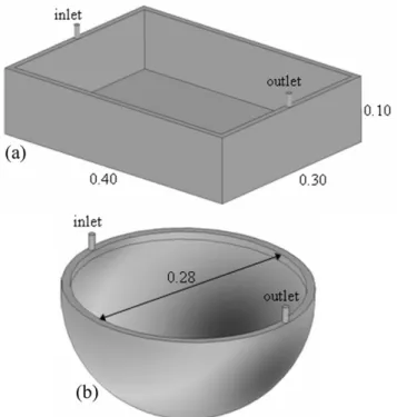
In this section, two 3D numerical simulations of the RTM process were also performed with FLUENT® and PAM-RTM® to validate the methodology developed in the FLUENT® code. The results showed that both simulations predicted the same flow front behavior and nearly the same filling time. Next, the LRTM process was simulated in FLUENT® to enable comparison between its obtained results and those for the RTM process. For this, the ability of the FLUENT® code to study parts which include porous media and open regions (channels) in the same simulation was explored, showing the relevance of this work. In these analyses, two different geometries were investigated, a rectangular box and a spherical shell (see Fig. 8).
Figure 8. Geometries for the RTM processes (in m): (a) Rectangular box and (b) Spherical shell.
In Fig. 8, the inlet and outlet cylindrical nozzles have diameter
of 8 10× −3m and height of 30 10× −3m. The wall thickness is
3
10 10× − m. The box was discretized using 129382 tetrahedral cells and the spherical shell was discretized using 66144 tetrahedral cells.
A porous medium with isotropic permeability K=3.89 10× −9m2
and porosity ε =0.88 was used, and the resin properties were
density ρ=916.00kg m/ 3 and viscosity µ=0.07115Pa s⋅ . For the
RTM process, an injection pressure of P=0.7 10× 5Pa was considered and the results for different filling times are presented for the rectangular box geometry shown in Fig. 9. The pictures on the left are the results obtained with PAM-RTM® and those on the right represent those obtained with FLUENT®.
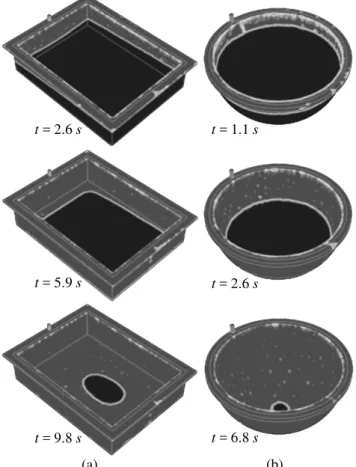
Figure 9. Rectangular box filling at time: (a) t = 81 s, (b) t = 181 s and (c) t = 343 s.
Figure 10. Spherical shell filling at time: (a) t = 17 s, (b) t = 92 s and (c) t = 189 s.
Based on the obtained results, two numerical simulations of the LRTM process were performed. The same geometries were adopted, although it was necessary to include a peripheral channel without porous medium (called border) and to alter the position of the outlet region to the central lower surface of the mold (Fig. 11). A gradient
pressure of ∆ =P 0.7 10× 5Pa between inlet and outlet regions was considered in both cases. The border thickness for the rectangular
box is 20 10× −3m and, for the spherical shell, 10 10× −3m.
Figure 11. Geometries for the LRTM process: (a) Rectangular box and (b) Spherical shell.
J. of the Braz. Soc. of Mech. Sci. & Eng. Copyright 2012 by ABCM April-June 2012, Vol. XXXIV, No. 2 / 111 Figure 12. LRTM processes: (a) Rectangular box filling and (b) Spherical
shell filling.
Final Remarks
Resin Transfer Molding (RTM) is a versatile process for the efficient manufacturing of composite materials with complex shapes and high structural performance. The numerical simulation of the mold filling stage in RTM is an important tool to assist the design of molds and to minimize the risk of producing defective parts.
A procedure for the modeling mold filling using the FLUENT® commercial code was used in present work. The Darcy’s Law and the Volume of Fluid (VOF) method are employed to predict the mold filling time and the flow front position. This procedure was compared with analytical, experimental and numerical (generated by PAM-RTM® software) results, showing a maximum variation of 8.12% and demonstrating the validity and effectiveness of the developed methodology.
In addition, a new approach for the numerical simulation of the Light Resin Transfer Molding (LRTM) process was developed in this work, demonstrating the viability of combining porous media regions with open (empty) regions, as found in the LRTM process. The simulations carried out showed the large difference in filling
pattern and required time for the complete filling of the same part when comparing RTM and LRTM processes.
Acknowledgements
The authors wish to thank CAPES (PROCAD), FAPERGS and CNPq for their financial support.
References
Ballata, W.O., Walsh, S.M. and Advani, S., 1999, “Determination of the Transverse Permeability of a Fiber Perform”, Journal of Reinforced Plastics and Composites, Vol. 18, No. 16, pp. 1450-1464.
Bejan, A., 2004, “Convection Heat Transfer”, Ed. John Wiley & Sons, 673 p.
Bruschke, M.V. and Advani, S.G., 1990, “A Finite-Element Control Volume Approach to Mold Filling in Anisotropic Porous-Media”, Polymer Composites, Vol. 11, No. 6, pp. 398-405.
FLUENT, 2008, “Documentation Manual – FLUENT 6.3”.
Hattabi, M., Echaabi, J. and Bensalah, O., 2008, “Numerical and Experimental Analysis of the Resin Transfer Molding Process”, Korea-Australia Rheology Journal, Vol. 20, No. 1, pp. 7-14.
Modi, D., Simacek, P. and Advani, S., 2003, “Influence of Injection Gate Definition on the Flow-Front Approximation in Numerical Simulations of Mold-Filling Processes”, International Journal for Numerical Methods in Fluids, Vol. 42, No. 11, pp. 1137-1248.
Morren, G., Bottiglieri, M., Bossuyt, S., Sol, H., Lecompte, D., Verleye, B. and Lomov, S.V., 2009, “A Reference Specimen for Permeability Measurements of Fibrous Reinforcements for RTM”, Composites Part A: Applied Science and Manufacturing, Vol. 40, pp. 244-250.
Nielsen, D.R., Pitchumani R., 2002, “Closed-Loop Flow Control in Resin Transfer Molding using Real-Time Numerical Process Simulations”,
Composites Science and Technology, Vol. 62, pp. 283-298. PAM-RTM, 2008, “User’s Guide & Tutorials”.
Rudd, C.D., 2005, “Liquid Moulding Technologies: Resin Transfer Moulding, Structural Reaction Injection Moulding, and Related Processing Techniques”, SAE International.
Schmidt, T.M., Goss, T.M., Amico, S.C. and Lekakou, C., 2009, “Permeability of Hybrid Reinforcements and Mechanical Properties of Their Composites Molded by Resin Transfer Molding”, Journal of Reinforced Plastics and Composites, Vol. 28, pp. 2839-2850.
Shojaei, A., Ghaffarian, S.R. and Karimian, S.M.H., 2004, “Three-Dimensional Process Cycle Simulation of Composite Parts Manufactured by Resin Transfer Molding”, Composite Structures, Vol. 65, pp. 381-390.
Silva, F.M.V., Souza, J.A., Rocha, L.A.O. and Amico, S.C., 2008, “Comparison of Two Numerical Methodologies for the Modeling of the RTM Process”, Proceedings of the 12th Brazilian Congress of Thermal Sciences and Engineering, Belo Horizonte, Brazil.
Souza, J.A., Nava, M.J.A., Rocha, L.A.O. and Amico, S.C., 2008, “Two-Dimensional Control Volume Modeling of the Resin Infiltration of a Porous Media with Heterogeneous Permeability Tensor”, Materials Research, Vol. 11, No. 3, pp. 267-268.
Souza, J.A., Rocha, L.A.O. and Amico, S.C., 2007, “Numerical Simulation of the Resin Transport through Fiber Reinforcement Medium”, Proceedings of the 19th International Congress of Mechanical Engineering,
Brasília, Brazil.
Yang, J., Jia, Y.X., Sun, S., Ma, D.J., Shi, T.F. and An, L.J., 2008, “Enhancements of the Simulation Method on the Edge Effect in Resin Transfer Molding Processes”, Materials Science and Engineering: A, Vol. 478, pp. 384-389.
t = 2.6 s t = 1.1 s
t = 2.6 s
t = 6.8 s t = 5.9 s
t = 9.8 s