Brazilian Journal of Physics, vol. 34, no. 4A, December, 2004 1469
Local Persistence and Blocking in the Two-Dimensional
Blume–Capel Model
Roberto da Silva
Departamento de Inform´atica Te´orica, Instituto de Inform´atica, Universidade Federal do Rio Grande do Sul Av. Bento Gonc¸alves, 9500, CEP 91501-970 Porto Alegre RS Brazil
and S. R. Dahmen
Inst´ıtuto de F´ısica, Universidade Federal do Rio Grande do Sul Av. Bento Gonc¸alves, 9500,CEP 90570-051 Porto Alegre RS Brazil
Received on 26 March, 2004. Revised version received on 27 July, 2004
In this paper we study the local persistence of the two–dimensional Blume–Capel Model by extending the concept of Glauber dynamics. We verify that for any value of the ratioα=D/J between anisotropyDand exchangeJthe persistence shows a power law behavior. In particular forα <0we find a persistence exponent
θl= 0.2096(13), i.e. in the Ising universality class. Forα >0(α6= 1) we observe the occurrence of blocking.
Among the many relevant quantities of interest in the modelling of nonequilibrium dynamics of spin systems such as first time passage [1], which has been extensively dis-cussed in the literature due to the appearance of non–trivial exponents in the power law behavior of the first return pro-bability as function of time, another quantity of interest is that of persistence, i.e. the characterization of the time it ta-kes for a particular spin not to change its state from its given
t= 0configuration. DefiningP(t)as the probability that a particular spin will not flip up to timet, at zero temperature temperature and for the Ising and Potts models this quantity was shown to behave as [2, 3]
P(t)∼t−θl, (1)
where the persistence exponent θl describes the
non-equilibrium relaxation of the system. This has been determi-ned through coarsening simulations since one expects that the fraction of spins which do not change up totrepresents a good estimate ofP(t). As a consequence one may intro-duced a global version of the concept of persistence through the quantityPg(t)which represents the probability that the
magnetization does not change its sign from itst = 0 va-lue, as done in [4]. Recently one of the authors explored these ideas to determine the associated θg exponent in the
Blume–Capel Model, in particular its behavior at the criti-cal and tricriticriti-cal points [8]. It was found that the exponent shows an abrupt change as one goes from the critical points (θg ≃0.23, Ising universality class) to the tricritical one.
The purpose of this letter is to extend Glauber’s dyna-mics to the Blume–Capel Model and to study the influence of the anisotropy on the exponentθl. For the sake of clarity,
we start with a brief overview of the Ising model.
AtT = 0the dynamics can be greatly affected by local
blocking configurations. Blocking is a phenomenon where a fraction of spins remains unchanged aftert Monte-Carlo simulation steps. The energy necessary to overcome them might be so high as to render the system static. On the other hand, forT 6= 0it becomes difficult to define domains be-cause one might not be able to distinguish between true do-mains and spin flips due to thermal fluctuations. Nonethe-less for the Ising Model these difficulties can be overcome and a power law decay for the fraction of persistent spins was found out in the whole low temperature phase [5]. The values found for the exponent wereθl= 0.22,0.22and0.29
forT = 0,T =Tc/3andT = 2Tc/3respectively.
Further-more forT > Tcan exponential cutoff was verified. Indeed,
using a natural definition of persistence, the effects of bloc-king are sensitive to any temperature value, and power law happens only atT = 0. The dynamics is implemented as follows: define the excitation energy∆Eassociated to the transitionσi → −σi as∆E =−2JσiSi, withSiequal to
the sum of nearest neighbors toσi. If∆E <0then the
tran-sition occurs with probability 1. For∆E= 0it occurs with probability1/2and the transition does not occur if∆E >0. All transition rules forT = 0are derived from the Glau-ber dynamics function atT >0, defined for 2-states models (i.e.S = 1/2) as:
w(σi→ −σi) =
1 2 ·
1−tanh µ ∆E
2kBT
¶¸
(2)
1470 Roberto da Silva and S. R. Dahmen
limitT →0
w(σi → −σi) T→0
→
1 if ∆E <0 1/2 if ∆E= 0 0 if ∆E >0
.
One of most important questions in nonequibrium dyna-mics is however whether theT >0extension of the dyna-mics from theT = 0case satisfies detailed balance:
w(σi→ −σi)/w(−σi→σi) = exp(−
∆E kBT
).
This condition is fulfilled by the Glauber dynamics ofq– state spin models.
To extend these ideas to the Blume–Capel Model we start out with the Hamiltonian
H =−JX
i
σiσi+1+D
X
i
σ2
i (3)
whereσi ∈ {−1,0,1}, J > 0 and D represents an
ani-sotropy. As we shall see the behavior of the persistence exponent is strongly dependent on the value ofα = D/J
yielding a nontrivial extension of the Ising Model. To imple-ment the Glauber dynamics in the ground state at (T = 0) we consider the excitation energy (in units of J ) for the transitionσi→σf as follows:
∆E/J= (σf−σi) [α(σf+σi)−Si] (4)
withSi ∈ [−4,4]∩Z. To go from theT = 0single spin
Glauber dynamics of a 2–state system to a 3–state model is not straightforward and some rules have to be introduced. Let the energy differences in the transition from σi to any
other two spin statesσ1
f orσ
2
f be represented by∆E1 and
∆E2respectively.
A simple dynamics that in the zero temperature li-mit of a Glauber dynamics satisfies detailed balance is the following: Choose betweenσ1
fandσ2fwith probability1/2,
for exampleσ1
f, then use theT →0limit of (2) to accept or
to reject the flipσi→σf1.
In our opinion however this is not the best choice, since it is biased in the sense that it does not make any distinction between situations as the following ones:
1. If∆E1<0and∆E2<0, a the transition to the state
with the smallest energy (the greater absolute energy gradient) will occur with probability 1, contrary to the rules of the simpler dynamics, where one chooses a state with probability1/2and apply theT = 0 dyna-mics as defined;
2. If∆E1= ∆E2 = 0, the transition must occur to any
state (σi, σf1orσ2f) with the same probability (1/3).
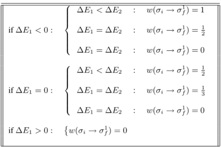
TABLE 1. Transition rules at T= 0 adoted for Blume–Capel Model
if∆E1<0 :
∆E1<∆E2 : w(σi→σ
1
f) = 1
∆E1= ∆E2 : w(σi→σf1) =
1 2
∆E1= ∆E2 : w(σi→σ
1
f) = 0
if∆E1= 0 :
∆E1<∆E2 : w(σi→σ
1
f) =
1 2
∆E1= ∆E2 : w(σi→σ
1
f) =
1
3
∆E1= ∆E2 : w(σi→σ
1
f) = 0 if∆E1>0 :
©
w(σi→σ
1
f) = 0
Thus more convenient rules should be defined in order to establish probability transitions that mimic the Blume– Capel Model atT = 0. We propose the following rule
w(σi→σ1f) = δξ(∆E1),−1
¡1
2δ∆E1,∆E2+δ1,ξ(∆E2−∆E1) ¢
+ δ0,ξ(∆E1) ¡1
3δ∆E1,∆E2+12δ1,ξ(∆E2) ¢ (5) where
ξ(x) =
1 ifx >0 0 ifx= 0 −1 ifx <0 andδx,yis Kronecker’s delta function.
For the sake of clarity all transitions envisaged by this rule are given in the table 1.
Do these probabilities arise from a function that satisfies detailed balance forT > 0?Otherwise one may have the impression that our dynamics is somewhat arbitrary and that our results do not reflect a fundamental property of Blume– Capel Model.
ForT > 0we propose a dynamics we call Metropolis– Gibbs sampling approach1:
w(σi→σ1 ,2
f ) =
exp(−∆E1,2
kBT )
1 + exp(−∆E1,2
kBT ) + exp(−
∆E2,1
kBT )
(6)
as a equivalent alternative to Glauber dynamics for the Blume–Capel Model atT >0
In the limitT →0all rules described in (table 1) can be obtained from this equation. Detailed balance is also gua-ranteed since
w(σi→σ1f) =
exp(−∆kB TE1)
1+exp(−∆kB TE1)+exp(−∆kB TE2)
and
w(σ1
f →σi) =
exp(∆E1
kB T)
1+exp(∆E1
kB T)+exp(
∆E1−∆E2 kB T )
,
1
Brazilian Journal of Physics, vol. 34, no. 4A, December, 2004 1471
once that
w(σi→σ1f)
w(σ1
f →σi)
= exp µ
−∆E1
kBT
¶ .
Finally with rules (table 1) Monte Carlo simulations were performed atT = 0on a square latticeL×L(L = 160) to measure the fraction of spins that do not flip during
t simulation steps. Since the sample numberNs does not
play an important role due to the absence of significant sta-tistical fluctuations (see e.g. [6]) we used Ns = 200with
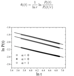
1000 MC steps. After some exploratory simulations a total of60different values ofαwithinα∈[−3,3]where chosen. After the 300th MC step convergence to power laws are found, as can be seen in Fig. 1. Forα <0we obtained the exponentθl = 0.214(3)by measuring directly the slope in
the interval[300,1000], with error bars obtained using 5 dif-ferent bins. A more precise estimate can be obtained using the definition of the effective exponent (local slope):
θl(t) =
1 lnrln
Pl(t)
Pl(t/r)
(7)
5.4 5.6 5.8 6.0 6.2 6.4 6.6 6.8 7.0 -2.6
-2.4 -2.2 -2.0 -1.8 -1.6
ln
P
(t)
α < 0
α = 0
α = 1
ln t
Figure 1. The numerical estimate of the probabilityP(t)in (1) as described in the text.
Forr = 10andt = 1000we obtainθl = 0.2096(13).
The same power law behavior was observed forα= 0and
α= 1, however with slightly different exponents, as can be seen in table 2.
TABLE 2. Local persistence exponent values of Blume–Capel Mo-del.
α <0 α= 0 α= 1
θl 0.2096(13) 0.1964(34) 0.1993(21)
For positive values ofα(6= 1) the system shows bloc-king, i.e., the fraction of spins that remain no changed aftert
Monte Carlo steps, as can seen in Fig. 2. However a distinc-tion must be made: inα∈]0,1[the persistence has a fast decay and reaches a constant value P(t → ∞) ≃ 0.322,
while forα ∈]1,2]the value isP(t → ∞) ≃0.246. For
α= 2,P(t → ∞)≃0.287) and whenα > 2there is full blocking withP(t → ∞)frozen to the value≃0.333 (ini-tial mean fraction of spins is null). Ind= 2andT = 0this is due to the fact that forα >2the predominant phase is a configuration with all spins zero.
1 10 100 1000
0.24 0.26 0.28 0.30 0.32 0.34
BLOCKING EFFECTS FOR α > 0
1 < α < 2
α = 2
α > 2
P
(t
)
t
Figure 2. Blocking effects for positive values ofα(6= 1).
Our values forα <0are in agreement with more recent results for the Ising Model, namely [7]
θl= 0.209(2) (8)
The pointα= 0separates two distinct regions: a power law behavior for negative values ofαand a blocking phase for positive values of this ratio. Atα= 0we have a power law behavior but with a different exponent.
Another interesting behavior is observed for α = 1, where a robust power law separates two different blocking ”phases”. The pointα= 2also divides two regions of dis-tinct blocking behavior: the1< α <2region and the full– blocking regionα >2.
To conclude, our results show that a nontrivial behavior in stochastic persistence can appear as one extends the Ising Model to allow for higher ”spins” and anisotropy effects as measured by our parameterα. In particular forα <0one has a pure 2–state Ising behavior; the same is not observed for different values ofα, as discussed in the text. It would be interesting to test these ideas in other stochastic systems in order to see whether some sort of nontrivial behavior might be found.
Acknowledgements
1472 Roberto da Silva and S. R. Dahmen
References
[1] W. Feller, An Introduction to Probability Theory and Its Ap-plications, 1, John Whiley & Sons (1968).
[2] B. Derrida, A. J. Bray, and C. Godr`eche, J. Phys. A 27, L357 (1994).
[3] D. Stauffer, J. Phys. A 27, 5029 (1994).
[4] S. N. Majumdar, A. J. Bray, S. J. Cornell, and C. Sire, Phys. Rev. Lett. 77, 3704 (1996).
[5] B. Derrida, Phys. Rev. E 55, 3705 (1997).
[6] S. Jain, Phys. Rev. E 59, 42493 (1999).
[7] S. Jain, H. Flynn, J. Phys. A 33, 8383 (2000).