Noncommutative Solitons and Instantons
Fidel A. Schaposnik
Departamento de F´ısica, Universidad Nacional de La Plata
Comisi´on de Investigaciones Cient´ıficas, Buenos Aires
C.C. 67 1900, La Plata, Argentina
Received on 21 October, 2003
I review different approaches to the construction of vortex and instanton solutions in noncommutative field theories.
1
Introduction
The development of Noncommutative Quantum Field Theo-ries has a long story that starts with Heisenberg observation (in a letter he wrote to Peierls in the late 1930 [1]) on the pos-sibility of introducinguncertainty relations for coordinates, as a way to avoid singularities of the electron self-energy. Peierls eventually made use of these ideas in work related to the Landau level problem. Heisenberg also commented on this posibility to Pauli who, in turn, involved Oppenhei-mer in the discussion [2]. It was finally Hartland Snyder, an student of Openheimer, who published the first paper on Quantized Space Time[3]. Almost immediately C.N. Yang reacted to this paper publishing a letter to the Editor of the Physical Review [4] where he extended Snyder treatment to the case of curved space (in particular de Sitter space). In 1948 Moyal addressed to the problem using Wigner phase-space distribution functions and he introduced what is now known as the Moyal star product, a noncommutative associ-ative product, in order to discuss the mathematical structure of quantum mechanics [5].
The contemporary success of the renormalization pro-gram shadowed these ideas for a while. But mathematici-ans, Connes and collaborators in particular, made important advances in the 1980, in a field today known as noncommu-tative geometry [6]. The physical applications of these ideas were mainly centered in problems related to the standard model until Connes, Douglas and Schwartz observed that noncommutative geometry arises as a possible scenario for certain low energy limits of string theory and M-theory [7]. Afterwards, Seiberg and Witten [8] identified limits in which the entire string dynamics can be described in terms of non-commutative (Moyal deformed) Yang-Mills theory. Since then, 1300 papers (not including the present one) appeared in thearXivdealing with different applications of noncom-mutative theories in physical problems.
Many of these recent developments, including Seiberg-Witten work, were triggered in part by the construction of noncommutative instantons [9] and solitons [10], solutions to the classical equations of motion or BPS equations of noncommutative theories. The present talk deals, precisely,
with the construction of vortex solutions for the noncommu-tative version of the Abelian Higgs model and of instanton solutions for noncommutative Yang-Mills theory. It covers work done in collaboration with D.H. Correa, G.S. Lozano, E.F. Moreno and M.J. Rodr´ıguez.
The plan of the talk is the following. In the next section I describe the construction of noncommutative field theories using the Moyal star product and how this can be connec-ted, in the case of even dimensional spaces, with a Fock space formulation. The approach will allow to turn the more involved non-linear equations of motion (or BPS equations) in noncommutative space into algebraic equations which are simpler to analyze. The application of this technique to the construction of vortex solutions in the noncommutative Abelian Higgs model is presented and finally, in the last sec-tion, instanton solutions to the self-dual equation for aU(2) noncommutative gauge theory are discussed.
2
The connection between Moyal
pro-duct of fields and operator propro-duct
in Fock space
Let us call xµ, µ = 1,2, ...d the coordinates of d -dimensional space-time. Givenφ(x)andχ(x), two ordinary functions inRd, their Moyal product is defined as [5]
φ(x)∗χ(x) = exp
µ
i
2θµν∂ µ x∂yν
¶
φ(x)χ(y)
¯ ¯ ¯ ¯
y=x
= φ(x)χ(x) + i 2θµν∂
µφ(x)∂νχ(x)
−18θµαθνβ∂µ∂αφ(x)∂ν∂βχ(x) +. . .(1)
withθµν a constant antisymmetric matrix of rank2r ≤ d and dimensions of(length)2. One can easily see that (1) defines a noncommutative but associative product,
Under certain conditions, integration overRdof Moyal pro-ducts has all the properties of the the trace (Tr) in matrix calculus,
Z
dx φ(x)∗χ(x) =
Z
dx χ(x)∗φ(x) =
Z
dx φ(x)χ(x) (3) Indeed, identity (3) holds when derivatives of fields vanish sufficiently rapidly at infinity, since
φ(x)∗χ(x) = φ(x)χ(x) + i 2θµν∂
µφ(x)∂νχ(x) − 1
8θµαθνβ∂µ∂αφ(x)∂ν∂βχ(x) +. . .
= φ(x)χ(x) +∂µΛµ
One has also in this case cyclic property of the star product,
Z
dx φ(x)∗χ(x)∗ψ(x) =
Z
dx ψ(x)∗χ(x)∗φ(x) (4)
Finally, Leibnitz rule holds
∂µ(φ(x)∗χ(x)) =∂µφ(x)∗χ(x) +φ(x)∗∂µχ(x) (5) The∗-commutator, denoted with[, ],
[φ, χ] =φ(x)∗χ(x)−χ(x)∗φ(x) (6) is usually called a Moyal bracket. If one considers the case in whichφandχcorrespond to space-time coordinatesxµ andxν, one has, from eq.(1),
[xµ, xν] =iθµν (7) This justifies the terminology “noncommutative space-time” although in the Moyal product approach to noncommutative field theories one takes space as the ordinary one and it is th-rough the star multiplication of fields that noncommutativity enters into play. For example, the action for a massive self-interacting scalar field takes, in the noncommutative case, the form
S=
Z
d4x
µ
∂µφ∗∂µφ−
m2 2 φ∗φ−
λ
4!φ∗φ∗φ∗φ
¶
(8) Note that due to eq.(3), the quadratic part of the action coin-cides with the ordinary one (and hence Feynman propaga-tors are the same for commutative and noncommutative the-ories). It is through interactions that differences arise.
We are interested in coupling scalars to gauge fields. Given a gauge connectionAµ and a gauge group element
g ∈ G, the gauge connection should transform, under a gauge rotation as
Ag
µ(x) =g(x)∗Aµ(x)∗g−1(x) +
i eg
−1(x)
∗∂µg(x) (9)
Note that even in the U(1) case, due to noncommutative multiplication, the second term in the r.h.s. has to be pre-sent in order to have a consistent definition of the curvature.
Also, the expression forg(x)as an exponential should be understood as
g(x) = exp∗(iǫ(x))≡1 +iǫ(x)−1
2ǫ(x)∗ǫ(x) +. . . (10) Accordingly, even in theU(1)case the curvatureFµν neces-sarily implies a gauge field commutator,
Fµν =∂µAν−∂νAµ−ie(Aµ∗Aν−Aν∗Aµ) (11) and then, as it happens for non Abelian gauge theories in ordinary space, the field strengthFµν is not gauge invariant but gauge covariant,
Fµν→g−1∗Fµν∗g (12) However, due to the trace property of the integral, the Maxwell action is gauge invariant,
S =1 4
Z
d4xF
µν∗Fµν (13)
As for matter fields, one can write
Df
µφ=∂µ+iAµ∗φ “fundamental” but also
Df¯
µφ=∂µ−iφ∗Aµ “anti−fundamental”
Dadµ φ=∂µφ−ie(Aµ∗φ−φ∗Aµ) “adjoint” (14) Extending non-Abelian gauge theories with generators
tato the noncommutative case is problematic. Consider for example the case ofG=SU(N). In the commutative case one has
[Aµ, Aν] = AaµAbνtatb−AbνAaµtbta
= AaµAbν
¡
tatb−tbta¢
| {z }
fabctc
(15)
so that the commutator, anda fortiorithe field strength, take values, as the gauge field itself, in the Lie algebra of the gauge group. In contrast, in the noncommutative case the presence of the star product prevents to arrange the commu-tator as above,
[Aµ, Aν] =Aaµ∗Abνtatb−Abν∗Aaµtbta
Using
tatb= 2if abctc+
2
NδabI+ 2dabct
c (17)
we see that
Fµν =(1)Fµνa ta+ (2)F
µνI (18)
3
Noncommutative solitons
In order to understand the difficulties and richness one en-counters when searching for noncommutative solitons, let us disregard the kinetic energy term in action (8) and just consider the scalar potential,
V[φ∗φ] = 1 2m
2φ
∗φ−λ
4φ∗φ∗φ∗φ (19) The equation for its extrema is
m2φ−λφ∗φ∗φ= 0 (20) or, with the shiftφ→(m/√λ)φ,
φ(x)∗φ(x)∗φ(x) =φ(x) (21) To find a solution, consider a functionφ0(x)such that
φ0(x)∗φ0(x) =φ0(x) (22) which evidently satisfies (21). Although simpler than (21), (22) implies, through Moyal star products, derivatives of all orders as it was the case for the original equation. Only some solutions can be found straightforwardly or with some little work. For example, ind= 2dimensions one finds
φ0 = 0
φ0 = 1
φ0 = 2 √
θexp
¡
−~x2/θ¢ −−→
θ→0 δ
(2)(x) (23)
Already a solution like (23) shows that nontrivial regular so-lutions, which were excluded in the commutative space due to Derrick theorem, can be found in noncommutative space. The the reason for this is clear: the presence of the parame-terθcarrying dimensions oflength2, prevents the Derrick scaling analysis leading to the negative results in ordinary space.
Finding more general solutions needs new angles of at-tack. A very fruitful approach was developed in [10] by exploiting an isomorphism between the algebra of functions with the noncommutative Moyal product and the algebra of operators on some Hilbert space. We shall describe this pro-cedure below in a simple two-dimensional example (but any even dimensional space can be treated identically).
We then start with two-dimensional space with complex coordinates
z=√1 2(x
1+ix2), ¯z= 1 √
2(x 1
−ix2) (24)
Changing the coordinate normalization, ˆ
a= √1 2θ(x
1+ix2), aˆ† =√1
2θ(x
1
−ix2) (25)
one ends with noncommutative coordinates satisfying [x1, x2] =iθ−→[ˆa,ˆa†] = 1 (26)
Thenˆaandaˆ† satisfy the algebra of annihilation and
crea-tion operators. One then considers a Fock space with a basis
|niprovided by the eigenfunctions of the number operator
N,
ˆ
N = ˆa†ˆa Nˆ|ni=n|ni (27) Note that one can establish a connection betweennand the radial variable,
ˆ
N = ˆa†ˆa≈ 1
2θ(x
2+y2) = r2
2θ, θ →0 (28)
Configuration space at infinity then corresponds ton→ ∞
in Fock space. Now, it is very easy to write projectorsPnin Fock space,
Pn =|nihn|, Pn2= 1 (29) so that
Pn3=Pn (30) which is nothing but the configuration space equation (21) for the minimum of the potential, but written in Fock space. So, we can say that we know a solution to (21) in operator form,
Oφ=|nihn| (31) Now, how does one pass from this solution in Fock space to the corresponding solution in configuration space? The answer is to use the Weyl connection which can be summa-rized as follows: given a fieldφ(z,¯z)in configuration space, take its Fourier transform
˜
φ(k,k¯) =
Z
d2zφ(z,z¯) exp
µ
i
θ(¯kz+kz¯)
¶
(32)
with variables defined as before,
z=√1 2
¡
x1+ix2¢ k=√1 2
¡
k1+ik2¢ (33)
¿From it, define the associated operator
Oφ(a, a†) = 1 4π2θ
Z
d2kφ˜(k,k¯) exp¡−i¯ka+ka†¢ (34)
Then, one can prove that
OφOχ
| {z }
operator product
=O φ∗χ
| {z }
∗product
(35)
Hence, the complicated star product of fields in configura-tion space becomes just a simple operator product in Fock space. As an example of how this connection can be used, consider the expression forPn (that can be found in any textbook on second quantization)
|nihn|=: 1
m!a† nexp(
−a†a)an : (36)
(Here “: :” means normal ordering) Then, Weyl connection implies
: 1
m!a
†n exp(
−a†a)an:
=
Z d2k 4π2φ˜
n
0(¯k, k) :e−i(kz¯a+kza
†)
or, anti-transforming (and using Rodrigues formula) ˜
φn
0(¯k, k) = 2πexp(−k2/2)Ln(k2/2) (37) whereLn is the Laguerre polynomial of ordern. Finally, Fourier transforming this expression, one can write in confi-guration space
φn
0(¯z, z) = 2(−1)nexp
³zz¯
θ
´
Ln
µ
2¯zz θ
¶
(38)
In this way, any operator solution in Fock space can be connected with the corresponding solution in configuration space where fields are multiplied using the star product. In particular, a general solution for the minimum of the poten-tial equation
φ(~x) =φ(~x)∗φ(~x)∗φ(~x) (39) ind= 2space is then,
in Fock space : Pφ =
X
λn|nihn|
in configuration space : φ = Xλnφn0(~x) (40) withλn= 0,±1andφn0 given by (38).
Now, we want more than solving equations for the ex-trema of potentials. We then have to be able to write kinetic energy terms in Fock space. To this end, observe that
[a†, an] =
−nan−1
(41) We then see that we can identify
∂f
∂a =−[a†, f(a)] (42)
so that derivatives of fieldsφbecome, in operator language,
∂zφ→ − 1 √
θ[a
†, O
φ], ∂z¯φ→ 1 √
θ[a, Oφ] (43)
and the Lagrangian associated to action (8) can be written in the form
L= 1 2
¡
[a, Oφ]2+ [a†, Oφ]2
¢
−m 2
2 O 2 φ+
λ
4O 4 φ (44) A last useful formula for the connection relates integration in configuration space with trace of operators in Fock space:
Z
dxdyφ(x, y) ⇒ 2πθTrOφ (45)
¿From here on we shall abandon the notationOφfor opera-tors and just writeφboth in configuration and Fock space.
4
Noncommutative vortices
The noncommutative version of the Abelian Higgs Lagran-gian (in the fundamental representation) reads
L=−1 4Fµν∗F
µν+D
µφ∗Dµφ−
λ
4(φ∗φ¯−η
2)2 (46)
Let us briefly review how vortex solutions were found in such a model in ordinary space [11]-[13]. The energy for static, z-independent configurations is, for the commutative version of the theory,
E= 1 2F
2
ij+DiφDiφ+
λ
4(|φ| 2
−η2)2 (47)
Herei = 1,2so one can consider the model in two dimen-sional Euclidean space with
Diφ=∂i−iAiφ , φ=φ1+iφ2 (48)
The Nielsen-Olesen strategy to find topologically non trivial regular solutions to the equations of motion of this model in ordinary space can be summarized in the following steps going from the trivial to the vortex solution:
1. Trivial solution
|φ|=η , Ai= 0 (49)
2. Topologically non-trivial but singular solution (flu-xon)
φ=ηexp(inϕ), Ai=n∂iϕ (50)
with
Z
d2xεijFij = 2πn (51)
but
εijFij = 2πnδ(2)(x) (52)
3. Regular Nielsen-Olesen vortex solution
φ=f(r) exp(inϕ), Ai=a(r)∂iϕ (53)
with boundary conditions:
f(0) =a(0) = 0, f(∞) =η , a(∞) =n (54)
4. Bogomol’nyi bound
ifλ= 2, E≥2πn (55)
whenever the following first order “Bogomol’nyi” equations hold
Fz¯z=η2−φφ¯ −Fz¯z=η2−φφ¯
Dz¯φ= 0 Dzφ= 0
Exact solutions of these equations can be easily construc-ted. Let us describe as an example the noncommutative self-dual case. One just copies the commutative strategy, starting from the “trivial” solution that we found in terms of projec-tors
|φ|=η
| {z }
trivial
⇒ φ=ηX fm
|{z}
0,±1 |mihm|
|φ|=ηexp(iϕ)
| {z }
singular
=η z
|z| ⇒ φ=η
X
fm|mihm|ˆa
|φ|=f(r) exp(iϕ)
| {z }
regular
=f z
|z| ⇒ φ=
X¯
fm|mihm|ˆa
(57)
Note that in the second and third lines we have used the iden-tificationz→(1/√θ)ˆa. The difference between these two formulæis that in the second the coefficients arefm =±1 while in the third one thefm¯ should be adjusted using the eqs. of motion and boundary conditions.
Of course (57) should be accompanied by a consistent ansatz for the gauge field,
ˆ
Az=
X
¯
enaˆ†|mihm| (58)
Differential equations (eqs. of motion or Bogomol’nyi eqs.) become algebraic recurrence relations which can be easily solved. For example, in the selfdual case one has from Bo-gomol’nyi equations
p
(n+ 2)(fn+1−fn)−enfn+1= 0 2p(n+ 1)en−1−e2n−1−2
p
(n+ 2)en−e2n =−θη2(fn2−1)
The appropriate condition at infinity (|z| → ∞) was, in con-figuration spacef(|z|) → 1. It translates tofn → 1 for
n→ ∞. Then, usingf0as a shooting parameter, one deter-minesf1, f2, . . .and from them one computes the magnetic field, the flux, the energy, from the expressions
B(r) = 2η2X∞ n=0
(−1)n¡1 −f2
n
¢
exp
µ
−r 2
θ
¶
Ln( 2r2
θ )
Φ = 2πθTr ˆB = 2π
E= 2πη2 (59)
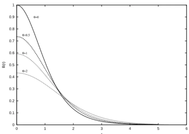
For smallθone re-obtains the Nielsen-Olesen regular vortex solution. Exploring the whole range ofθη2, the dimension-less parameter governing noncommutativity, one finds that the vortex solution with+1units of magnetic flux exists in all theθ range. As an example, we show in Figure 1 the magnetic field of a self-dual vortex with N = 1units of magnetic flux, for different values ofθ. We see that the so-lution approaches smoothly the commutative (θ= 0) limit.
0 0.1 0.2 0.3 0.4 0.5 0.6 0.7 0.8 0.9 1
0 1 2 3 4 5 6
B(r)
r
θ=0
θ=0.5
θ=1
θ=2
Figure 1. Magnetic field of a self-dual vortex as a function of the radial coordinate (in units ofη) for different values of the anticom-muting parameterθ(in units ofη2). The curve forθ= 0coincides with that of the Nielsen-Olesen vortex in ordinary space.
In the commutative case, anti-selfdual solutions can be trivially obtained from selfdual ones by makingB → −B,
φ → φ¯. Now, the presence of the noncommutative para-meterθ, breaks parity and the moduli space for positive and negative magnetic flux vortices differs drastically. One has then to carefully study this issue in all regimes, not only forλ= λBP Sbut also forλ6= λBP S, when Bogomol’nyi equations do not hold and the second order equations of mo-tion should be analyzed. A summary of results which are obtained is (see details in ([18],[19],[22]):
• Positive flux
1. There are BPS and non-BPS solutions in the whole range ofη2θ. Their energy and magne-tic flux are:
For BPS solutions
EBP S = 2πη2N , Φ = 2πN
N = 1,2, . . . (60) For non-BPS solutions,
Enon−BP S > 2πη2N , Φ = 2πN
N = 1,2, . . . (61) 2. For η2θ → 0 solutions become, smoothly, the known regular solutions of the commutative case.
3. In the non-BPS case, the energy of anN = 2 vortex compared to that of twoN = 1vortices is a function ofθ.
As in the commutative case, if one compares the energy of anN = 2vortex to that of twoN = 1 vor-tices as a function ofλone finds that forλ > λBP S
N >1vortices are unstable (vortices repel) while for
• Negative flux
1. BPS solutions only exist in a finite range: 0≤η2θ≤1
Their energy and magnetic flux are:
EBP S = 2πη2N , Φ = 2πN
N = 1,2, . . . (62) 2. Whenη2θ= 1the BPS solution becomes a flu-xon, a configuration which is regular only in the noncommutative case. The magnetic field of a typical fluxon solution takes the form
B∼√1 θexp(r
2/θ)
−−→
θ→0 δ
(2)(x) (63)
3. There exist non-BPS solutions in the whole range ofθbut
(a) Only forθ <1they are smooth deformati-ons of the commutative ones.
(b) Forθ →1they tend to the fluxon BPS so-lution.
(c) Forθ > 1they coincide with the non-BPS fluxon solution.
5
Noncommutative instantons
The well-honored instanton equation
Fµν =±F˜µν (64) was studied in the noncommutative case by Nekrasov and Schwarz [9] who showed that even in theU(1)case one can find nontrivial instantons. The approach followed in that work was the extension of the ADHM construction, succes-sfully applied to the systematic construction of instantons in ordinary space, to the noncommutative case. This and other approaches were discussed in [29]-[38]. Here we shall des-cribe the methods developed in [31],[35].
We work in four dimensional space where one can always choose
θ12=−θ21=θ1
θ34=−θ43=θ2 all otherθ′s= 0
We define dual tensors as ˜
Fµν = 1 2
√g ε
µναβFαβ (65)
withgthe determinant of the metric.
In order to work in Fock space as we did in the case of noncommutative vortices, we now need two pairs of creation annihilation operators,
x1 ±ix2
⇒ ˆa1, ˆa1†
x3±ix4 ⇒ ˆa2, ˆa2†
and the Fock vacuum will be denoted as|00i. Concerning projectors the connection with configuration space takes the form
|n1n2ihn1n2| ⇒ exp¡−r12/θ1−r22/θ2¢Ln1
¡
2r21/θ1¢×
Ln2
¡
2r22/θ2¢ (66) Finally, note that the gauge groupSU(2)(for which ordi-nary instantons were originally constructed) should be re-placed byU(2)so that
Aµ =Aaµ
σa 2 +A
4 µ
I
2 (67)
Let us now analyze how the different ansatz leading to ordinary instantons can be adapted to the noncommutative case.
1- (Commutative)’t Hooft multi-instanton ansatz (1976)
Aµ(x) = ˜Σµνjν
˜ Σµν =
1 2η¯aµνσ
a, η¯ aµν=
εaµν , µ, ν6= 4
δaµ, ν = 4 −δaν , µ= 4
jν=φ−1∂νφ
Hereσa are the Pauli matrices (’t Hooft ansatz corresponds to anSU(2)gauge theory). With this ansatz, the instanton selfdual equation becomes
Fµν = ˜Fµν ⇒ 1
φ∇φ= 0 (68)
with
φ= 1 + N
X
i=1
λ2 i (x−ci)2
, ∇φ= N
X
i=1
δ(4)(x
−ci) (69)
The solution corresponds to a regular instanton of topologi-cal chargeQ=N.
2- Noncommutative version of ’t Hooft ansatz
The natural way of extending ’t Hooft ansatz is to pro-ceed with the changes
jν =φ−1∂νφ ⇒ jν=φ−1∗∂νφ+∂νφ∗φ−1
Aa µ
σa
2 = ¯Σµνjν ⇒ A a µ
σa
2 = ¯Σµνjν (70)
A4µ =−i¡φ−1
∗∂νφ−∂νφ∗φ−1
¢
(71) With this we see that the Poisson equation (69) for ordinary instantons changes according to
1
φ∇φ= 0 ⇒ φ
−1
∗ ∇φ∗φ−1= 0
∇φ=δ(4)(x)⇒ ∇φ= λ 2
θ1θ2|
One then gets, for the field strengths,
F = ˜F+|00ih00| (73) We see that the self-dual equation is not exactly satisfied: the|00ih00|term, the analogous to the delta function in the ordinary case, is not cancelled as it happened with the delta function source for the Poisson equation (68) in the commu-tative case.
3- Noncommutative BPST (Q= 1) ansatz (1975)
The pioneering Belavin, Polyakov, Schwarz and Tyup-kin ansatz [39] leading to the firstQ= 1instanton solution was similar to the ’t Hooft ansatz except thatΣµν was used instead of its dualΣ˜µν. Its noncommutative extension can be envisaged as
Aaµ
σa
2 = Σµνjν ⇒ A a µ
σa
2 = Σµνjν (74) wherejν is defined as in the previous ansatz. Concerning
A4
µ, the consistent ansatz changes due to the use ofΣµν ins-tead of its dual as in the ’t Hooft ansatz. One needs now, instead of (71),
A4µ=i¡φ−1
∗∂νφ+ 3∂νφ∗φ−1
¢
(75) With this, one finally has
Fµν = ˜Fµν , Q=S= 1 (76) but, due to the necessity of the consistent ansatz for theA4 µ component, one can see that
Fµν 6=Fµν† (77) and hence the price one is paying in order to have a selfdual field strength is its non-hermiticity. Note however that the action and the topological charge are real.
4- (Commutative) Witten ansatz (1977)
The clue in this ansatz [40] is to reduce the four di-mensional problem to a two didi-mensional one through an axially symmetric N-instanton ansatz. That is, one passes from 4 dimensional Euclidan space to 2 dimensional space, (x1, x2, x3, x4
→r, t) but this last with a nontrivial metric
gij =r2δij, i, j= 1,2.
The axially symmetric ansatz for the gauge field compo-nents is
~
Ar = Ar(r, t)Ω(~ ϑ, ϕ)
~
At = At(r, t)Ω(~ ϑ, ϕ)
~
Aϑ = φ1(r, t)∂ϑΩ(~ ϑ, ϕ)
+ (1 +φ2(r, t))Ω(~ ϑ, ϕ)∧∂ϑΩ(~ ϑ, ϕ)
~
Aϕ = φ1(r, t)∂ϕ~Ω(ϑ, ϕ)
+ (1 +φ2(r, t))Ω(~ ϑ, ϕ)∧∂ϕ~Ω(ϑ, ϕ) (78)
with
~
Ω(ϑ, ϕ) =
sinϑcosϕ
sinϑsinϕ
cosϑ
(79)
With this ansatz, the selfduality instanton equation (64) becomes a pair of BPS equations for vortices in curved space
Fµν = ˜Fµν →
½ 1
√gFzz¯=|φ|2−1
Dzφ= 0
(80)
where φ = φ1 +iφ2 and z = t +ir. Solving these BPS vortex equations then reduces to finding the solution of a Liouville equation. In this way an exact axially sym-metry N-instanton solution was constructed in [40] for the (commutative)SU(2)theory.
4-Noncommutative version of Witten ansatz
To proceed, one needs a noncommutative setting for cur-ved 2-dimensional space, whereθ can in principle depend onx,
[xi, xj] =θij(x) (81) Now, handling such a commutator is not trivial since not all functionsθij(x)will guarantee a noncommutative but asso-ciative product.
One can see, however, that associativity can be achieved whenever
∇iθij= 0 (82)
In the present 2 dimensional case, these equations have as solution
θij=θ0
εij
√g (83)
withθ0 a constant. Then, given the metric in which the instanton problem with axial symmetry reduces to a vortex problem we see that an associative noncommutative product should take the form
[r, t] =r2θ
0; all other[., .] = 0 (84) with nowrandtdefining the two dimensional variables in curved space. A further simplification occurs after the ob-servation that
r∗t−t∗r=r2θ0 ⇒ t∗ 1
r−
1
r ∗t=θ0 (85)
Then, callingy1 = t andy2 = 1/r we have instead of (84) the usual flat space Moyal product and the Bogomol’nyi equations take the form
µ
1−1 2(z+ ¯z)
2
¶
Dzφ =
µ
1 +1 2(z+ ¯z)
2
¶
Dz¯φ(86)
iFz¯z = 1− 1
2[φ,φ¯]+ (87)
iFz¯z = − 1
2[φ,φ¯] (88) withz=y1+iy2. We can at this point apply the Fock space method detailed above for constructing vortex solutions. In the present case, consistency of eqs.(86)-(88) imply
¯
and hence the only kind of nontrivial ansatz should lead, in Fock space, to a scalar field of the form
φ=X n=0
|n+qihn| (90)
whereqis some fixed positive integer. With this, it is easy now to construct a class of solutions analogous to those pre-viously found for vortices in flat space. It takes the form
φ = X n=0
|n+qihn|
Az = −
i
√
θ0 q−1
X
n=0
¡√
n+ 1¢|n+ 1ihn|+
+ √i
θ0
X
n=q
³p
n+ 1−q−√n+ 1´|n+ 1ihn|
(91) One can trivially verify that configurations (91) satisfy eqs.(86)-(88) providedθ0 = 2. In particular, both the l.h.s. and r.h.s of eq.(86) vanish separately. The field strength as-sociated to our solution reads, in Fock space,
iFzz¯=− 1
2(|0ih0|+. . .+|q−1ihq−1|)≡B (92) or, in the original spherical coordinates
~
Ftu = B(r)~Ω
~
Fϑϕ = B(r) sinϑ ~Ω
Ftu4 = B(r)
F4
ϑϕ = B(r) sinϑ (93) As before, starting from (92) forB in Fock space, we can obtain the explicit form of B(r)in configuration space in terms of Laguerre polynomials, using eq.(66). Concerning the topological charge, it is then given by
Q = 1 32π2tr
Z
d4xεµναβF µνFαβ
= 1
π
Z 0
−∞
du
Z ∞
−∞
dtB2= 2TrB2= q 2 (94) We thus see that Q can be in principle integer or semi-integer, and this for an ansatz which is formally the same as that proposed in [40] for ordinary space and which yielded in that case to an integer. The origin of this difference between the commutative and the noncommutative cases can be tra-ced back to the fact that in the former case, boundary con-ditions were imposed on the half-plane and forced the so-lution to have an associated integer number. In fact, if one plots Witten’s vortex solution in ordinary space in the whole (r, t)plane, the magnetic flux has two peaks and the corres-ponding vortex number is even. Then, in order to parallel this treatment in the noncommutative case one should im-pose the conditionq= 2N.
Acknowledgements: I would like to thank the organizers of the XXIV Encontro Nacional de F´ısica de Part´ıculas e
Campos at Caxambu for inviting me to deliver a talk at such an impressive meeting and for their warm hospitality. This work is partially supported by UNLP, CICBA, ANPCYT, Argentina.
References
[1] SeeWolfgang Pauli, Scientific Correspondence, Vol II, p.15, Ed. Karl von Meyenn, Springer-Verlag, 1985.
[2] See Wolfgang Pauli, Scientific Correspondence, Vol III, p.380, Ed. Karl von Meyenn, Springer-Verlag, 1993.
[3] H.S. Snyder, Phys. Rev.71, 38 (1947).
[4] C. N. Yang, Phys. Rev.72, 874 (1947).
[5] J. E. Moyal, Proc. Cambridge Phil. Soc.45, 99 (1949).
[6] A. Connes, Noncommutative geometry, Academic Press, New York, 1994.
[7] A. Connes, M. R. Douglas, and A. Schwarz, JHEP9802, 003 (1998).
[8] N. Seiberg and E. Witten, JHEP9909, 032 (1999).
[9] N. Nekrasov and A. Schwarz, Commun. Math. Phys. 198, 689 (1998).
[10] R. Gopakumar, S. Minwalla, and A. Strominger, JHEP0005, 020 (2000).
[11] H. B. Nielsen and P. Olesen, Nucl. Phys. B61, 45 (1973).
[12] H. J. de Vega and F. A. Schaposnik, Phys. Rev. D14, 1100 (1976).
[13] E. B. Bogomolny, Sov. J. Nucl. Phys.24, 449 (1976); [Yad. Fiz.24, 861 (1976)].
[14] D. P. Jatkar, G. Mandal, and S. R. Wadia, JHEP0009, 018 (2000).
[15] A. P. Polychronakos, Phys. Lett. B495, 407 (2000).
[16] J. A. Harvey, P. Kraus, and F. Larsen, JHEP0012, 024 (2000).
[17] D. Bak, Phys. Lett. B495, 251 (2000).
[18] G. S. Lozano, E. F. Moreno, and F. A. Schaposnik, Phys. Lett. B504, 117 (2001).
[19] G. S. Lozano, E. F. Moreno, and F. A. Schaposnik, JHEP
0102, 036 (2001).
[20] A. Khare and M. B. Paranjape, JHEP0104, 002 (2001).
[21] D. Bak, K. M. Lee, and J. H. Park, Phys. Rev. D63, 125010 (2001).
[22] G. S. Lozano, E. F. Moreno, M. J. Rodriguez, and F. A. Scha-posnik, Non BPS noncommutative vortices, arXiv:hep-th/0309121.
[23] K. Hashimoto and H. Ooguri, Phys. Rev. D 64, 106005 (2001).
[24] O. Lechtenfeld and A. D. Popov, JHEP0111, 040 (2001).
[25] R. Gopakumar, M. Headrick, and M. Spradlin, Commun. Math. Phys.233, 355 (2003).
[26] F. Franco-Sollova and T. A. Ivanova, J. Phys. A 36, 4207 (2003).
[27] D. Tong, J. Math. Phys.44, 3509 (2003).
[29] K. Furuuchi, Prog. Theor. Phys.103, 1043 (2000).
[30] A. Schwarz, Commun. Math. Phys.221, 433 (2001).
[31] D. H. Correa, G. S. Lozano, E. F. Moreno, and F. A. Scha-posnik, Phys. Lett. B515, 206 (2001).
[32] S. Parvizi, Mod. Phys. Lett. A17, 341 (2002).
[33] K. Y. Kim, B. H. Lee and H. S. Yang, Phys. Lett. B523, 357 (2001).
[34] O. Lechtenfeld and A. D. Popov, JHEP0203, 040 (2002).
[35] D. H. Correa, E. F. Moreno, and F. A. Schaposnik, Phys. Lett. B543, 235 (2002).
[36] F. Franco-Sollova and T. A. Ivanova, J. Phys. A36, 4207 (2003).
[37] Z. Horvath, O. Lechtenfeld, and M. Wolf, JHEP0212, 060 (2002).
[38] T. A. Ivanova and O. Lechtenfeld, Phys. Lett. B567, 107 (2003).
[39] A. A. Belavin, A. M. Polyakov, A. S. Shvarts, and Y. S. Tyup-kin, Phys. Lett. B59, 85 (1975).