Attitude Determination for Low Cost IMU and Processor Board
using the Methods of TRIAD, Kalman Filter and Allan Variance
Mayara Mesiano Carrasco 1, [email protected] André Luís da Silva 2
1
Universidade Federal do ABC, Santo André, SP 2
Universidade Federal de Santa Maria, Cachoeira do Sul, RS
Submetido em 13/09/2015
Revisado em 15/10/2015 Aprovado em 01/03/2016
Resumo: Este artigo apresenta métodos para determinação de atitude usando sensores MEMS e um processador de baixo custo Arduino One. Filtros de Kalman foram desenvolvidos para fundir os dados de acelerômetro, magnetômetro e giroscópio. Os dados do acelerômetro e magnetômetro foram processados com o método de TRIAD. As matrizes de covariância usadas no projeto dos filtros de Kalman foram obtidas pela análise de variância de Allan dos sensores. Um filtro de Kalman foi melhorado com uma modelagem de ruído do giroscópio que combina o ruído branco padrão com o random walk. Resultados experimentais mostram que esta mudança pode determinar resultados razoavelmente diferentes em relação aqueles do filtro de Kalman padrão.
Palavras chave: Navegação Inercial, Filtro de Kalman, Determinação de Atitude, Variância de Allan.
Abstract: This paper presents methods for attitude determination using low cost MEMS sensors and an Arduino One board. Kalman filters were developed to fuse the data of accelerometer, magnetometer and gyroscope. Accelerometer and magnetometer data were processed using the TRIAD method. The covariance matrices used in Kalman filter design were obtained from Allan variance analysis. One Kalman filter was improved using a random walk noise combined with the standard white noise in the gyroscope. Experimental results showed that this augmented filter can generate results reasonably different from that of the standard Kalman filter.
1. Introduction
Navigation is an ancient art that became a complex technique. Generally speaking, navigation is the determination of position, velocity and attitude (angular orientation) of a body with respect to a fixed reference frame (FRF). One of the most popular navigation techniques is related to the observation of well known fixed points, e.g. the stars. Nowadays, other kind of navigation is well spread, which is based on movable space stations, i.e. satellites. There are three operational global navigation satellite systems (GNSS): GPS (EUA), GLONASS (Russia), GALILEO (EU). GNSS have global coverage and can determine reasonable accurate data [1] of position and velocity, however, the acquisition of attitude data is not straightforward.
On the other hand, an inertial navigation system (INS) is an alternative to the GNSS. An INS is composed by an inertial measurement unit (IMU), which is attached to the body, and a processing unit. An IMU is composed by inertial sensors that detect the following physical quantities: the accelerometer measures the specific force (inertial acceleration less gravitational acceleration) in the body reference axes, or body reference frame (BRF); the gyroscope measures the angular velocity in the BRF. An IMU can have additional sensors, such as the magnetometer, that measures the local magnetic field along the BRF. The processing unit has a microprocessor that performs signal processing and executes algorithms for the determination of position, velocity and attitude (PVAT) from the sensor data. Theoretically, and INS can determine accurate estimates of PVAT, however, time correlated noises can degrade its performance, [2].
An accurate INS has high cost, however, in the last decades, low cost miniature inertial sensors have been developed: micro-electro-mechanical-systems (MEMS). MEMS accelerometers, gyroscopes and magnetometers are well spread in many INS, they enable many day by day applications such as mobile phones and low cost robotics. However, these sensors, in general, have low accuracy and can degrade the estimation of PVAT [3].
This paper presents the application of some techniques for improving the accuracy of an INS for attitude determination using MEMS sensors. The attitude is determined from magnetometer and accelerometer measurements using the
TRIAD (triaxial attitude determination) method, [4]. A Kalman filter is applied for improving the estimation in the presence of noise, combining the results of TRIAD with gyroscope data. The Allan variance technique is used to characterize the noise of the inertial sensors, giving more detailed information to design the Kalman filter. This development was applied to a low cost IMU with MEMS sensors and an Arduino One processing board.
The remaining of this paper is divided as folows: section 2 provides a general view of attitude representation, attitude determination, Kalman filter and Allan variance, section 3 describes the process of sensor data error modeling and Kalman filter design, section 4 shows the experimental setup, experimental results and discussion, section 5 summarizes the main conclusions taken from the experimental work.
2. Theoretical Basis 2.1 Attitude Representation
The attitude of a rigid body can be defined as the orientation of a BRF with respect to a set of 3 orthogonal axes attached to a suitable reference system. In most applications, the reference frame is the NED (north, east, down), where the x, y and z axes point to the local north, east and down directions, respectively, [5]. The orientation between two reference frames can be parameterized in many forms. One of the most intuitive and straightforward is the 3x3 transformation matrix, or direction cosine matrix (DCM), that converts a vector from one reference frame to another. A second form is the set of Euler angles that represents 3 successive rotations from one system to another. The most popular set of Euler angles involve the roll, pitch and yaw angles ( , and , respectively). Another important attitude parameterization is the quaternion, which is a vector of four components related to an instantaneous axis of rotation and a rotation angle, obtained from the Euler rotation theorem. Each attitude representation can be more suitable for a given problem and one can be converted into another. In this work, the DCM, quaternion and Euler angles were considered, depending on the situation.
The attitude kinematics describes the time evolution of the attitude from the angular velocity. Given the quaternion, the rotational kinematics is determined
by, [5]: ˙ = , = 0 − − − 0 − − 0 − 0 (1)
where = [ ] is the quaternion, and = [ ] is the angular velocity vector, which is written in the BRF (T means the transpose). The attitude kinematics can be written in any parameterization, the main advantage of choosing the quaternion is the linearity of the equation and the reduced number of terms.
If the DCM is known, the quaternion can be obtained by the conversion:
= , = , = , = ± 1 + + + (2)
where is the element in the row i and column j of the DCM (rotation matrix from the FRF the BRF).
2.2 TRIAD
The DCM can be determined from at least two vector observations. The simplest method of attitude determination from vector observations is the TRIAD [4]. If two pairs of unitary vectors are written as and in the FRF, and and
in the BFR, then, by definition:
= , = (3)
where is the DCM. This equation can be used to determine from the two pair of vectors. However, its solution is not unique, in fact, it depends on weights in the pairs 1 or 2. The TRIAD method states that, a balanced solution (which is called TRIAD3) is given by:
= + + ( × )( × ) , =
| |, =| |
(4)
where and are defined similarly, “×” is the cross product operator, | | is the modulus a vector .
2.3 Kalman Filter
The Kalman filter is a state estimator that observes the state vector of a system from output measurements, in the presence of measurement noise. A differential equation is necessary which describes the time evolution of the state
in the presence of process noise. The theory of Kalman filter is described in many textbooks, some of them focusing in applications, e.g. [1]. A short summary is given below.
The original version of Kalman filter only considers linear systems. The extended Kalman filter (EKF) is an adaptation for the case of nonlinear dynamic systems represented by:
̇ ( ) = ( , ( ), ) + ( , ) ( ) (5) where ∈ ℝ is the state, : [0, ∞) → ℝ is a given driving function, : ℝ × ℝ × [0, ∞) → ℝ is a vector valued nonlinear state function. ( ) ∈ ℝ is called process noise, it is a white Gaussian process with zero mean and covariance ( ) ∈ ℝ × , the process noise covariance matrix. : ℝ × [0, ∞) → ℝ × is a matrix valued nonlinear function called process noise distribution matrix.
The measurements are state dependent and represented by the nonlinear output function:
( ) = ( ) + ( ) (6)
where ∈ ℝ is the vector of measured outputs, : ℝ → ℝ is a vector-valued nonlinear output function. ( ) ∈ ℝ is called measurement noise, it is a white Gaussian process with zero mean and covariance ( ) ∈ ℝ × , the measurement noise covariance matrix.
The Kalman filter is generally implemented in the discrete time form. The main notation adopted is the following:
- : sampling interval, the time length between two consecutive state estimations;
- : k-th sampling time;
- : predicted state at time k ( ); - : corrected state estimate at time k;
- : predicted error’s covariance matrix at time k;
- : corrected error’s covariance matrix estimate at time k.
The following procedure composes the k-th iteration of the EKF. An initial estimate is needed, as usual, the method assumes that the initial state is distributed according to a white Gaussian noise with zero mean.
Prediction of the state vector:
= + ∫ ( ( ), ( ), ) (7)
Prediction of the error’s covariance matrix: ̇ ( ) = ( ) + ( ) +
=
= ( , ) ( ) ( , )
= + ̇ ( )
(8)
Correction (measurement update) Kalman gain:
= [ + ]
=
(9)
Correction of the state estimate:
= + [ − ( )] (10) Correction of the error’s covariance matrix estimate:
= − (11)
In equation (7), the vector function ( ) is given by data determined from measurement, e.g. gyroscope. In equation (10), is the output measured by another instrument at time k, e.g. accelerometer and magnetometer.
2.4 Allan Variance and Sensor Noise Characterization
MEMS sensors can manifest stochastic errors, which may be unsteady and time correlated. In this case, the modeling of these errors can be performed by the Allan variance [6].
Random noises do not have a well defined mathematical function, but some statistical properties can be defined, according to the theory of stochastic processes. The total noise can be decomposed as the summing of several noises of different nature, each one having some parameters for its characterization. In
an inertial sensor, the main components of noise are [3]: quantization, Gaussian white noise, random walk, flicker noise, exponentially correlated (Markov) and rate ramp. The Allan variance technique can be applied to identify each portion of noise generated by a sensor and also to quantify their parameters.
In the classical statistics, the variance is applied as a measure of dispersion, quantifying the how much some data spreads around a central point. This technique is useful when the data are stationary and do not posses time correlation. If this scenario is not valid, the Allan variance can be more appropriate.
The Allan variance consists in a time domain process developed for the study of frequency stability of oscillators. It can be related to the spectral density of the signal. This correspondence is the key for identifying the different components of a sensor noise.
Given a time sequence of a given signal with N points and sample time ts, the Allan variance consists in the division of this set according to subsets (groups) with n consecutive points. Each group is associated to a time interval T=n.ts, also called cluster time. This group has a mean value S(T). Then, the Allan variance of the subset of size n taken from the set of size N is given by [3]:
( ) =
( )∑ ( ̅ ( ) − ̅ ( )) (12)
where ̅ ( ) is the mean value of the k-th subgroup of n points (n=T/ts).
The method of modeling a sensor noise consists in collecting the data of the sensor when it is stationary. Then, the Allan variance is determined for different values of T, obtaining the Allan variance as a function of cluster time. These results are drawn as a log-log plot and some asymptotes are evaluated to identify the noise components and their parameters, [3].
3. Method
The concepts of section 2 were applied to develop attitude determination methods for an IMU with MEMS sensors.
The TRIAD method can be applied to determine the DCM from vector measurements of magnetometer and accelerometer. The FRF is the NED. The vector unitary is the acceleration due to gravity (g); after normalization, the result (in the NED frame) is simply: = [0 0 1] . The measurement is the
acceleration due to gravity in the BRF (with normalization). The accelerometer can measure the specific force in the BRF, given by: = − , where and are the body’s inertial acceleration and acceleration due to gravity written in the BRF. If the inertial acceleration is very small when compared to g, one can suppose that the accelerometer only measures –gb, this is assumed in this work.
The second vector used for attitude determination (unitary vector ) is given from the Earth magnetic field (geomagnetic field). The geomagnetic field varies with position and time in the Earth atmosphere. There are many models that estimate this field, the most popular are WMM (World Magnetic Model)1 and IGRF (International Geomagnetic Reference Field)2. In these models, the input data are the latitude, longitude, altitude and time, the result is the local geomagnetic field in the NED reference frame; the units are given in nT (nano Testa), then, can be computed with a simple normalization. On the other way, the normalized vector is measured in the BRF using the magnetometer. In this case, it is assumed that the magnetometer only measures the geomagnetic field. However, residual magnetization of the body and sensor can corrupt this measurement. In such a case, calibration is necessary. Methods of magnetometer calibration can be found in reference [7]. Even if a calibration is done, the sensor should not operate in environments where other fonts of magnetic fields are present. So, the assumption is made that only the geomagnetic field is active in the environment.
The gyroscopic sensor measures angular velocity in the BRF. Then, the attitude kinematics shall be used to compute the attitude. In this paper, the quaternion parameterization of equation (1) is used. The quaternion can be converted for DCM or Euler angles using standard formulae found in textbooks. Note that the attitude kinematics needs an external initial condition. So, the initial attitude shall be known, otherwise, this method will only compute variations. This initial value can be determined by the TRIAD.
Note that the TRIAD method and the attitude kinematics determine different estimates of the same physical quantity. Also, in practice, accelerometers, magnetometers and gyroscopes are corrupted by noise, as
1 https://www.ngdc.noaa.gov/geomag/WMM/DoDWMM.shtml 2 http://www.ngdc.noaa.gov/IAGA/vmod/igrf.html
discussed in section 2.4. In this kind of situation, the Kalman filter is used to perform sensor fusion in order to determine the best estimate in the presence of Gaussian white noise. However, as discussed in section 2.4, the Gaussian white noise is not the unique font of error in MEMS sensors. According to reference [3], after the Gaussian white noise, the second most important noise is the random walk. Fortunately, the random walk can be generated as the integral of a white noise. So, the Kalman filter equations can be augmented with an additional state variable that represents the random walk, with an additional input representing its generating white Gaussian noise.
In this paper, two Kalman filters were developed. The first one only considers white Gaussian noises. The state update is performed by the attitude kinematics (equation (1)) using angular velocity measurement from the gyroscopic sensor. The state update is performed from the attitude calculation performed by the TRIAD method, which receives data from the accelerometer and magnetometer. The processes noise covariance matrix (Q) is constant and determined from the variance of the gyroscopic sensor white noise; it is a diagonal 3x3 matrix. The measurement noise covariance matrix (R) is constant and determined from an estimate of the errors in the TRIAD method, which depends in the white Gaussian noises of the accelerometer and magnetometer; it is a diagonal 4x4 matrix.
Note that the attitude kinematics represents the attitude in means of quaternion, while the TRIAD determines the DCM. In order to use the TRIAD results in the update phase of the Kalman filter, the equation (2) is applied to convert the TRIAD results from DCM to quaternion.
The second filter is an extension of the first, where a random walk noise is assumed in each channel (three axes) of the gyroscopic sensor. So, the noises assumed in the gyroscope will be standard white Gaussian noise and random walk. In this situation, the Kalman filter will be improved with 3 state variables in the state propagation equation. These new states represent the integral of white noises that generate the random walk. The processes noise covariance matrix is also augmented. It will be a 6x6 diagonal matrix. The first 3 elements in the main diagonal are the variances of the gyroscope white noise, while the remaining 3 elements are the variances of the white noises that generate the random walk.
4. Results and Discussion
The experimental setup is composed as follows.
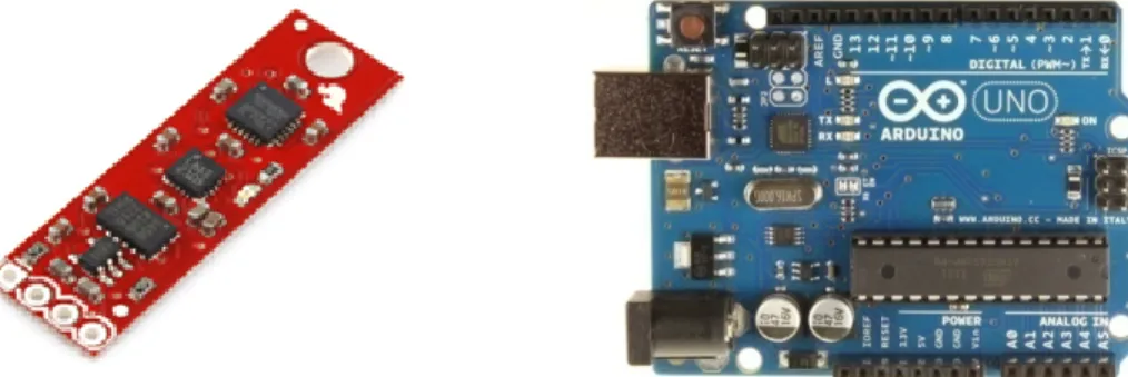
IMU board with MEMS sensors Sparkfun SEN-107243 containing: 3 axes gyroscope, 3 axis accelerometer and 3 axes magnetometer. Arduino UNO4 microprocessor board with ATmega 328P. The IMU and microprocessor communicate via I2C protocol. Figure 1 shows the IMU and Arduino boards.
Figure 1: Sparkfun SEN – 10724 and Arduino One.
PC computer with Intel core I3 processor running Windows 7. The Arduino microprocessor and computer communicate via USB 2.0. The Arduino board is programmed using its own open-source Arduino IDE5. The Arduino board
receives the data from the IMU and sends it to the PC via USB. The MATLAB® 2014 software is used to read and process the data in the PC.
The experimental procedures consist of two main activities:
(1): Characterization of the sensor noises using the Allan variance; (2): Implementation and tests of attitude determination methods. 4.1 Characterization of the sensor noises using the Allan variance
The sensor board was kept static and data was obtained for 4 hours. The sample time was ts = 0.02s, corresponding to 50Hz. 720,000 data samples were obtained (N=720,000 in Allan variance calculations). Each data sample is
3 https://www.sparkfun.com/products/10724 4 http://arduino.cc/en/Main/arduinoBoardUno 5 https://www.arduino.cc/en/Main/Software
composed by 9 measurements, 3 for each sensor. Although the data was collected for 4 hours, the maximum time T=n.ts was set to 1 hour for Allan variance analysis, in order to reduce the errors in large data sets [3]. The data were received in the PC via USB port and processed using MATLAB, where the Allan variance method was implemented.
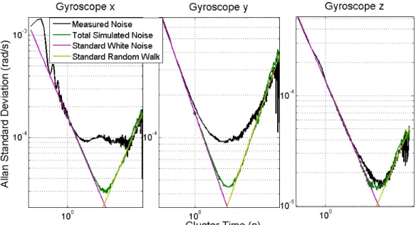
The detailed explanation about Allan variance analysis is performed in another paper. Figure 2 presents a general plot for the gyroscope. This figure is a log-log plot of Allan standard deviation (square root of Allan variance) against time. Results are shown for the 3 gyroscope axes: original data, simulated noises and theoretical standard noises. Simulated noises were generated using MATLAB for validating the approach.
Figure 2: Log-log plot of Allan standard deviation of the gyroscope.
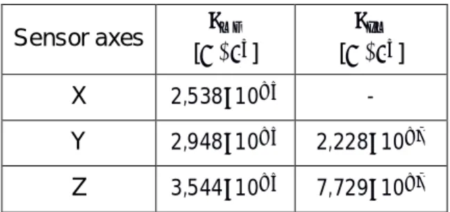
The Allan variance approach led to the identification of the main noises of accelerometer and gyroscope. In general, the most important noises are the white noise and the random walk. Table 1 presents the noise parameters for the accelerometer. Table 2 gives the noise parameters for the gyroscope. In these tables, the second column shows the standard deviation of white noise, the third column shows the standard deviation of the white noise that generates the random walk. Note that the random walk was not identified in the x axis of the accelerometer.
Sensor axes
[ ⁄ ] [ ⁄ ]
X 2,538 10 -
Y 2,948 10 2,228 10
Z 3,544 10 7,729 10
Table 2: Coefficients of the noises identified in the gyroscope.
Sensor axes
[ ⁄ ] [ ⁄ ]
X 1,121 10 3,873 10
Y 1,046 10 8,669 10
Z 9,539 10 1,019 10
4.2. Implementation and tests of attitude determination methods
The attitude determination methods were implemented in MATLAB and Arduino. Arduino data is processed in real time and sent to the computer. MATLAB is used for post-processing.
The standard Kalman filter described in section 3 was programmed in Arduino. TRIAD method and the attitude kinematics alone were also developed and tested in Arduino. However, all of them cannot run at the same time in the Arduino processor. The same algorithms were implemented in MATLAB, in order to validate the Arduino programs.
The Kalman filter augmented with random walk was programmed and tested only in MATLAB, because this augmentation compromises the Arduino processing.
During implementation, the sensor data (scale factor, sensitivities, etc) were taken from the respective data sheets. Magnetometer calibration parameters were obtained according the procedures explained in reference [7].
The attitude estimation algorithms run at 40Hz in Arduino and MATLAB. The process noise covariance matrices were built from data of Table 2. The measurement noise covariance matrix is diagonal with covariances equal to 10 , this is a roughly estimate from the data of table 1.
- The IMU was set to initial conditions close to zero: almost leveled, in order to get roll ( ) and pitch ( ) angles close to zero; heading close to north, in order to obtain yaw angle ( ) almost zero;
- Three maneuvers were performed rotating the IMU manually: yaw rotation close to 90°, pitch rotation close to 45°, roll rotation close to 45°;
- The same rotations were performed in the opposite order, trying to return the IMU to the original initial condition.
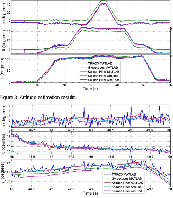
During the maneuver, the Arduino board computed the attitude and sent the data to the computer. After, the data was post-processed in MATLAB for validation. Figure 3 presents some results for one of these tests: roll, pitch and yaw angles. The Arduino board estimates the attitude in the quaternion form, but these data were converted to Euler angles before the generation of the figures, because Euler angles are better for visualization. Five results are shown:
- Standard Kalman filter that runs in real time in Arduino;
- MATLAB post processing: standard Kalman filter, Kalman filter augmented with random walk in gyroscope, TRIAD, attitude kinematics using gyroscope.
Several discussions can be developed from figure 3. The TRIAD method is the one that generate the noisiest results. This happens because no filtration is performed by this method. Instantaneous measurements from accelerometer and gyroscope determine instantaneous attitude values. But, note that the TRIAD method can determine the initial condition of the IMU ( ≅ −5,1°, ≅ −8,2°, ≅ 6°);
The gyroscope results are biased with respect to the others. This is expected, because the attitude kinematics starts from zero initial conditions. However, note that these results have less noise with respect to the TRIAD. In most MEMS sensors applications, the integration of gyroscope errors can generate divergence in the attitude calculation. However, in the time horizon of this experiment, the results have good behavior, without divergence;
Kalman filter results are a kind of weighted average between the attitude kinematics and TRIAD. In time 5 seconds, the estimation begins and the Kalman filter quickly corrects their estimates from its initial state using the TRIAD results. Then, the Kalman filter starts to perform estimates close to the TRIAD, but, with
a smaller level of noise.
Figure 3: Attitude estimation results.
Figure 4: Close view of some estimation results.
Figure 3 cannot show much difference between the 3 Kalman filter results. In this way, figure 4 presents a close view in some time interval. Because these experiments concern stochastic data, it is very difficult to establish general conclusions from specific cases. However, figure 4 can help one to understand some qualitative behavior. Different from what one could expect, the same program that runs in MATLAB and Arduino do not determine the same result.
That is: the standard Kalman filter that runs in real time in Arduino and the post processing in MATLAB do not determine equal paths in figure 4. Also, this discrepancy is not constant, sometimes increases, sometimes decreases. The most probable reason is the numeric methods implemented in MATLAB and Arduino. MATLAB software has good computational performance running in a 64 bits computer. On the other way, Arduino microprocessor has only 16 bits, corresponding to numeric representation of smaller precision. However, in the scenario of the limitation of the Arduino microprocessor, the results seem reasonable.
Figure 4 also shows that the two Kalman filters implemented in MATLAB (standard and augmented with random walk) do have different responses. Looking all the angles, in the sample interval shown, the difference is roughly between 0.5 and 6 degrees. It is not easy to demonstrate which estimate is better. This can be done with an additional measurement of a more accurate sensor. However, qualitatively, it is possible to argue that the insertion of random walk in the Kalman filter can determine reasonably different results.
5. CONCLUSION
This paper presents methods for attitude determination from MEMS sensors using a low cost processor. An Arduino One board was used to read a low cost MEMS IMU and compute attitude estimation algorithms.
The method TRIAD was used to determine attitude from accelerometer and magnetometer measurements. The integration of quaternion kinematics was used to compute the attitude from gyroscopic measurements. These two methods were fused using the Kalman filter.
A standard Kalman filter and an augmented Kalman filter were studied. The augmented filter has additional state variables that represent the random walk in the gyroscope. Allan variance technique was used in order to identify and determine the parameters of the noises present in the sensors.
Experimental results showed that the Arduino One board is suitable to run the estimation algorithms up to 40Hz. However, the augmented Kalman filter compromises the computational performance. But the other algorithms can run with reasonable precision when compared to the results given by a standard PC
computer.
The experimental results also shown that the augmentation of the Kalman filter with gyroscope random walk noise can generate significant differences in the attitude estimation results. However, additional tests are recommended to investigate the exact influence of these changes in the accuracy.
References
[1] GREWAL, Mohinder S. et al. Global Positioning systems, inertial navigation and integration. 2. ed. Hoboken, USA: Wiley-Interscience, 2007.
[2] TITTERTON, D. H.; WESTON, J. L. Strapdown inertial navigation technology. 2 ed. Reston, USA: AIAA, 2004.
[3] EL-SHEIMY, N.; HOU, H.; NIU, X. Analysis and modeling of inertial sensors using allan variance. IEEE Transactions on Instrumentation and Measurement, v. 57, n. 1, 140-149, 2008.
[4] MARKLEY, F.L. Attitude determination using two vector measurements. NASA
techdoc_19990052720, Goddard Space Flight Center, 1998, url:
http://www.archive.org/details/nasa_techdoc_19990052720
[5] TEWARI, A. Atmospheric and space flight dynamics: modeling and simulation with MATLAB and Simulink. Boston: Birkhäuser, 2007.
[6] CARVALHO, A. Influência da Modelagem dos Componentes de Bias - Instabilidade dos Sensores Inerciais no Desempenho do Navegador Integrado SNI GPS. Dissertação de Mestrado. Instituto Militar de Engenharia. Rio de Janeiro, 2011. [7] de Amorim, J. Estudo e aplicação de algoritmos computacionais para a calibração de magnetômetros. Dissertação de Mestrado. Universidade Federal do ABC. Santo André-SP. 2012.