GPS Interference Mitigation Using Derivative-free Kalman Filter-based RNN

DOI: 10.13164/re.2016.0518 SIGNALS

GPS Interference Mitigation

Using Derivative-free Kalman Filter-based RNN

Wei-Lung MAO

Graduate School of Engineering Science and Technology and Dept. of Electrical Engineering, National Yunlin University of Science and Technology, Taiwan

wlmao@yuntech.edu.tw

Manuscript received September 12, 2015

Abstract. The global positioning system (GPS) with accu-rate positioning and timing properties has become integral part of all applications around the world. Radio frequency interference can significantly decrease the performance of GPS receivers or even completely prohibit the acquisition or tracking of satellites. The approaches of system perfor-mances that can be further enhanced by preprocessing to reject the jamming signal will be investigated. A recurrent neural network (RNN) predictor for the GPS anti-jamming applications will be proposed. The adaptive RNN predictor is utilized to accurately predict the narrowband waveform based on an unscented Kalman filter (UKF)-based algo-rithm. The UKF algorithm as a derivative-free alternative to the extended Kalman filter (EKF) in the framework of state-estimation is adopted to achieve better performance in terms of convergence rate and quality of solution. The adaptive UKF-RNN filter can be successfully applied for the suppression of interference with a number of different narrowband formats, i.e. continuous wave interference (CWI), multi-tone CWI, swept CWI and pulsed CWI, to emulate realistic circumstances. Simulation results show that the proposed UKF-based scheme can offer the supe-rior performances to suppress the interference over the conventional methods by computing mean squared predic-tion error (MSPE) and signal-to-noise ratio (SNR) improvements.

Keywords

Global positioning system (GPS) receiver, narrowband interference, direct sequence spread spectrum (DSSS), recurrent neural network (RNN) predictor, unscented Kalman filter (UKF) algorithm

1.

Introduction

The global positioning system (GPS) [1] can provide accurate positioning and timing information useful in many applications. There is an increasing interest in positioning techniques based on GPS and cellular network infrastruc-ture or on the integration of the two technologies for

a wide spread of applications, such as tracking systems, navigation, and intelligent transportation systems. The satellites supply service to consumers around the world by using direct sequence spread spectrum (DSSS) modulation method. GPS spreads the bandwidth of transmitting signals with coarse/acquisition (C/A) code, which results in a 43 dB processing gain. DSSS technique inherently exhib-its a modest anti-jamming property that can cope with narrowband interference. Therefore, it is necessary to develop additional techniques for protection of the GPS in jamming environments.

lin-earizes all nonlinear transformations of state equation and measurement equation, substitutes Jacobian matrices for the linear transformations in the KF equations. It is recog-nized to be inadequate due to the linearization scheme [9]. Recently, Julier and Uhlmann [9] have introduced a new filter founded on the intuition that it is easier to approxi-mate a Gaussian distribution than it is to approxiapproxi-mate arbi-trary nonlinear functions. They named this filter as un-scented Kalman filter (UKF). The UKF leads to more accu-rate results than EKF and in particular it geneaccu-rates much better estimates of the covariance of the state.

In this paper, we study the performance of the UKF-based RNN predictors for stationary and nonstationary interference cancellation in GPS receivers. Since the inter-fering signals may not be stationary, a substitute model based on recurrent neural network (RNN) structure is more suitable for nonstationary signal prediction [8], [10]. The UKF can outperform the EKF in terms of prediction and estimation error, at an equal computational complexity for general state-space problems. Once the prediction of the jamming signal is obtained, an error signal can be com-puted by subtracting the estimate from the received signal. The error signal is then fed into the correlator for de-spreading.

The remainder of this paper is organized as follows. System model of received jamming signals is constructed in Sec. 2. Design of UKF-based neural network is de-scribed in Sec. 3. Simulation results are demonstrated in Sec. 4. Some conclusions are stated in the last section.

2.

Proposed System Models

GNSS systems are continuously going through pro-gressive evolution in the field of positioning and naviga-tion. A receiver computes its position, velocity and time solution by processing received data from a constellation of satellites. The radio frequency interference becomes the most disruptive operation of GPS receivers. Unfortunately, the low level of GNSS signal is susceptible to many types of interference, which can be either intentional or uninten-tional. This interference can significantly degrade the qual-ity of, or totally disable some of, the processes in the GPS receivers.

The satellites broadcast ranging codes and navigation data at two frequencies: primary L1 and secondary L2. Only the L1 signal, free for civilian use, will be considered. A simplified block diagram of an anti-jamming GPS model is shown in Fig. 1. The direct sequence spread spectrum signal is given by

1 ( ) 2 ( ) ( ) cos(2 _L )

s t  Pd t c t f t (1) where P is the signal power, d(t) is the 50-bps navigation data sequence, c(t) is the C/A code sequence with a chip-ping rate of 1.023 MHz, and fL1 is L1 carrier frequency

(1575.42 MHz). T is the coherent integration time, Tc is the

chip duration of ranging code, and the integer PG = T/Tc = 20460 (i.e. 43 dB) is the processing gain of the GPS

system. The received signal r(t) can be modeled as

( ) ( ) ( ) ( )

r t s t n t I t (2)

where n(t) is additive white Gaussian noise (AWGN) with variance 2, and the narrowband jamming source I(t) has a bandwidth much smaller than the GPS spreading band-width. The received signal is bandpass filtered, amplified and down converted. Due to the down-conversion, the spectrum of the signal is shifted to the baseband frequency. To further simplify the analysis, the received signal is as-sumed to pass through a filter matched to the chip wave-form and is sampled synchronously once during each chip interval. The observation becomes

( ) ( ) ( ) ( )

r k s k n k I k (3)

where {s(k)}, {n(k)}, and {I(k)} are discrete time sampled waveform of {s(t)}, {n(t)}, and {I(t)}, respectively. They are assumed to be mutually independent. The n(k) can be modeled as band-limited and white, and the jamming source being considered has a bandwidth much narrower than 1/Tc. The s(k) sequence is d(k)c(k) taking values of 1.

The low power jamming signal can be suppressed by GPS receivers with the 43 dB processing gain. However, if strong jamming signals are presented, they can result in degradation of navigation accuracy or even complete loss of receiver tracking. In this paper, four kinds of narrow-band interference will be considered:

(a) Single tone continuous wave interference (CWI)

a( ) cos( c )

I k I kT   (4)

where I is amplitude and  is its frequency offset from the center frequency of the spread spectrum signal. Tc is the

chip duration, which is equal to the sampling interval.  is a random phase uniformly distributed over the interval [0, 2).

(b) Multi-tone CWI

b c

1

( ) cos[ ]

N

i i i

i

I t I kT







where Ii, i, and i represent amplitude, random phase,

and frequency offset, respectively, of the i-th interferer from the central frequency of spread spectrum signal, and N is the number of narrowband interferers.

(c) Pulsed CWI

 

c T T 1

T 1 T

cos( ) ( 1) ( 1)

0 ( 1)

I k

I kT l N k l N N

l N N k lN





        

 _{   }



1, 2, 3,...

t

L1

cos

(a)

t

L1

cos

2 



0



(b)

Fig. 1. GPS spread spectrum system: (a) Transmitter. (b) Anti-jamming receiver.

where the on-interval is N1Tc seconds long and off-interval

is (NT – N1)Tc seconds long. We consider the case in which

NT and N1 are much greater than unity.

(d) Periodically swept (linear FM) CWI

2 d( ) cos[ ( 1) c 0.5 ( c) ]

I k I   l kT  kT   ,

(l1)K k lK l, 1, 2, 3,... (7) where I and  are the amplitude and random phase of the swept CWI.  represents the offset from the GPS carrier frequency,  is the sweep bandwidth,  = /K is the fre-quency rate, and K is the sweep period.

In Fig. 1(b), the narrowband canceller composed of an RNN predictor and an adder is employed to suppress the jamming signals. The predictor/subtractor implementation essentially produces a replica of the narrowband interfer-ence Î(k) which can be subtracted from the received signal to enhance the wideband components. The {s(k)} and {n(k)} sequences are wideband signals with nearly flat spectra. Thus, these two sequences cannot be estimated from their past values. The prediction of the GPS received signal using the adaptive nonlinear predictor based on previously received values will, in effect, be an estimate of the inter-fering signal. The interinter-fering signal {I(k)} can be predicted because of its correlated property. The error signal z(k) is obtained as

ˆ

( ) ( ) ( ) ( ) ( ) ( ) ( )

z k s k n k I k I k s k n k (8) where z(k) can be viewed as an almost interference-free signal and is fed into the correlator.

3.

Proposed Recurrent Neural

Net-work (RNN) Predictor

The prediction of a time series is synonymous with modeling of physical systems responsible for its generation.

However, the jamming signals always have statistically stationary/nonstationary properties, and the nonlinear structure suitable for estimation is the artificial neural network. RNNs are the most general type of neural net-works. They have feedback, a property which makes them capable of learning on-line and adapting to statistical varia-tion of incoming time series. RNNs have been proven [8] to be better than traditional signal processors in modeling and predicting nonlinear and chaotic time series, as well as in a wide variety of applications ranging from speech pro-cessing to adaptive channel equalization.

3.1

Recurrent Neural Network Dynamics

The detailed structure of an RNN is illustrated in Fig. 2. It has a neural module and a comparator of its own. Specifically, the module consists of a fully connected RNN with N hidden neurons, P external input neurons, and one output neuron. In each neuron, one-unit delayed version outputs of hidden neurons are assumed to be fed back to the input. Besides the P + N inputs, one bias input whose value is always at +1 is included. Let matrix Wa denote the

synaptic weights of the N neurons in the hidden layer that are connected to the feedback nodes in the input layer, and matrix Wb represent the synaptic weights of these hidden

neurons that are connected to the input nodes. It is further assumed that the bias term of hidden neurons are absorbed in the weight matrix Wb. The weight matrices Wa and Wb

can be expressed as

T a a1 ... a ... a

T T T

j N

 

  

W W W W , (9)

T b b1 ... b ... b

T T T

j N

 

  

W W W W , (10)





a b  1 ... j ... N

 _{  }

W W W W W W (11)

where Wa, Wb and W are N-by-N, N-by-(P + 1) and

) 1 (k r 1 ) 1 k ( qN 

) 1 k ( r  ) k ( q2 ) 1 k (

q1  () ( 1)

^

 rk k y ) (k e + -) k (

q1 wi,j

) k ( qN

I

z

) (k r   ) 1 (kP r

 

np lay r i n lay r O p lay r

) 1 k ( q2 

Fig. 2. Proposed recurrent neural network predictor.

Wj are defined by

aj  wa ,1j ... wa ,j N

W , (12)

bj wb ,1j wb ,j P1

W  , (13)

T

a _b

j  j _j

W W W . (14)

A (P + 1)-by-1 input vector R(k) can be constructed in terms of GPS observation samples r(k), r(k – 1),…, r(k – P + 1), and a bias input (+1). Let the N-by-1 vector

Q(k) denote the state of vector of an RNN, and the 1-by-1 vector y(k) denotes the corresponding output of the system. These vectors can then be described as

T ( )k [1, ( ), (r k r k1),..., (r k P 1)]

R , (15)

T 1

( )k [ ( ),...,q k qN( )]k

Q . (16)

Based on the definition above, an input vector consisting of the total (P + N + 1) input signal can be represented as

T

T T

( )k   ( )k ( )k _

U Q R . (17)

The dynamic behavior of an RNN can be described by the following pair of nonlinear state space equations:





T

T T T

1

( 1) ( ) ( )

( ( )) ( _j ( )) ( _N ( )) ,

k k k

k k k

  

 

 _   _

Q Φ W Q W R

W U  W U  W U

(18) ( )k  ( )k

y CQ (19)

where C is a 1-by-N matrix, which represents the synaptic weights of the output node connected to the hidden neu-rons, and : RN RN is a diagonal map,

1 1 2 2 ( ) ( ) ( ) N N x x x x x x        _   _        _      Φ

  (20)

with ( ) tanh( / 2) (1 ax) (1 ax)

x a x e e

      .

The nonlinear function (·) represents the sigmoid activation function of a hidden neuron, and a is the gain of a neuron. Any EKF-based training algorithm is a second order, recursive procedure that is particularly effective in training both recurrent and feedforward neural network architectures for a wide variety of problems. It typically requires fewer training cycles than does its RTRL [7] coun-terpart and tends to yield superior input-output mapping. This neural network training problem is viewed as a par-ameter estimation problem, and the synaptic weights are the parameters to be estimated. The unscented Kalman filtering is a derivative free alternative to EKF method for state estimation. The UKF method can utilize a determinis-tic sampling approach to calculate mean and variance terms. The dynamic behavior of an RNN can be modeled as the nonlinear discrete time state equations:

1 k  k  k

x x u , (21)

 

k  k  k

y H x v (22)

where xk is an N(N + P + 1)-by-1 vector obtained by

rearranging the weight matrix W(k) into a column vector, and yk is an N-by-1 observation vector. The first equation

states that the state of the neural network is represented as a stationary process corrupted by process noise uk. The

second equation, known as the observation equation, repre-sents the desired response vector yk as a nonlinear function

of weight vector xk and measurement noise vk. The

N(N + P + 1)-by-1 process noise vector uk, which has the

PDF uk ~ N(0,Ru), is independent from sample to sample,

so that E[um unT] = 0 for m n (vector WGN). vk. is

an N-by-1 observation noise vector with PDF vk ~ N(0,Rv),

and is independent from sample to sample; thus

E[vm vnT] = 0 for m n (vector WGN).

3.2

Node Decoupled Kalman Filter (NDEKF)

Learning Algorithm

The practical application of the EKF algorithm is lim-ited by its computational complexity. It has greater compu-tational complexity and storage requirements than the RTRL algorithm. As the EKF-based algorithm is domi-nated by storing and updating the error covariance matrix

Mk, the NDEKF learning algorithm is proposed here in

order to reduce the computational burden of the GEKF inherent in processing large matrices. The NDEKF algo-rithm divides the weights of the RNN into several groups of smaller size, with the weights grouped by output node, and the interaction between weight estimates can be ig-nored. This simplification introduces many zeros into ma-trix Mk. Therefore, the weights are decoupled so that the

weight groups are mutually exclusive of one another; as a result, Mk can be rearranged into block-diagonal form.

1, 2, , k k k g k             

M 0 0

0 M 0

M

0 0 M

     



(23)

where g denotes the total number of groups, and matrix

Mi,k is the weight conditional error covariance matrix of the

i-th group. The global gradient matrix Hk also needs to be

rearranged, so the weight vectors x̂(k) corresponding to a given output node neuron are grouped as a single block. Hence, the Hk is composed of individual submatrices Hi,k;

that is

1, 2, ,

k   k k g k

H H H  H . (24)

Based on the simplifying assumption above, the NDEKF algorithm for the i-th group can be expressed as

1 1       _

 g

i T k , i k , i k , i v i

k R H M H

A , (25)

, , ,

T i k  i k i k k

G M H A , i1, 2,...,g, (26)





, , ,

ˆi k  ˆi k i k k  (ˆk)

x w G y h x , i1, 2,...,g, (27)

, 1 , , ,

u i k   i k i k i k i

M I G H M R , i1, 2,...,g (28) where Ak is the global scaling factor required to compute

the Kalman gain matrix for all weight groups. For group i, the vector Gi,k is the Kalman gain of neurons, Hi,k is the

gradient matrix of each weight with respect to each output node, and vector x̂i,k refers to the estimated weights. The

concatenation of vector x̂i,k forms the vector x̂k. The matrix Riv is a diagonal measurement noise covariance matrix, and Riu is an additional positive process noise matrix.

3.3

UKF Learning Algorithm

The unscented transform is a method for calculating the statistics of a random variable which undergoes a non-linear transformation. Consider propagating a random variable X (dimension equal to L) through a nonlinear function Y = f(X). Assume X has mean X̅ and covariance

Px. To calculate the statistics of Y, we form a matrix χ of

2L + 1 sigma vector χi according to the following:

0

χ x, (29)

( ( ) )

i  L  x i

χ x P , i = 1,…,L, (30)

( ( ) )

i  L  x i L

χ x P , i = L + 1,…, 2L (31) where = α2(L + ) – L is a scaling parameter. The con-stant α determines the spread of the sigma points around X̅, and is usually set to a small positive value. The constant is a secondary scaling parameter, which is usually set to (3 – L). ( (L )P_x)_i is the i-th column of the matrix

square root. These sigma vectors are propagated through the nonlinear function

Υ_i f( )_i (32)

where the mean and covariance matrices for Y are approxi-mated using a weighted sample mean and covariance of the posterior sigma points,

2 ( m) 0 L i i i W  



y , (33)

2 (c) T y 0 ( )( ) L

i i i

i W







P y y (34)

with weights Wi given by

( m ) 1

0 ( )

W    L  , (35)

(c) 1 2

0 ( ) 1

W    L      , (36)

( m ) (c) 1 1 2 ( )

i i

W W   L   , i1,..., 2L. (37) The unscented Kalman filter is a straightforward ex-tension of the UT to the recursive estimation, where the state RV is redefined as the concatenation of the original state and noise variables: xka= [xkTukTvkT]T. The UT sigma

point selection scheme is applied to this new augmented state random variable to calculate the corresponding sigma matrix χka. The UKF equations are described further. Note

that no explicit calculations for Jacobians or Hessians ma-trices are necessary to implement this algorithm. Further-more, the overall number is of the same order as the EKF. The UKF algorithm is represented as follows:

(1) Initialize with xˆ₀ E

 

T 0 ( 0ˆ0)( 0ˆ0) 

P E x x x x , (38)

T

a a T

0 0

ˆ    _{  } ˆ _

x E x x 0 0 , (39)

0

a a a a a T u

0 0 0 0 0

v ˆ ˆ ( )( )        _   _{ } _    

P 0 0

P E x x x x 0 R 0

0 0 R

(40)

for k





(2) Calculate the sigma points:

a a a a a a

1 ˆ 1 ˆ 1 ( ) 1 ˆ 1 ( ) 1

k  k k  L  k k  L  k 

χ x x P x P .

(41) (3) The time-update equations: Each sigma point is propagated through the linear process model of RNN. It is expressed as

/ 1 1.

x x

k k  k

χ χ . (42)

2

( m) x , / 1 0

ˆ

L

k i i k k i W    



x χ , (43)

2

(c) x x T u

, / 1 , / 1 0

ˆ ˆ

( )( )

L

k i i k k k i k k k i W       



P χ x χ x R . (44)

The sigma points are propagated through the nonlinear observation model of RNN. It is given as





x x n

/ 1 / 1, 1 k k  k k k

y H χ χ , (45)

2

( m) x , / 1 0

ˆ

L

k i i k k i W    



y y . (46)

(4) The measurement-update equations: From the re-sulted transformed observations, the mean, covariance, and cross-covariance matrices are computed.

2

(c) T v

, / 1 , / 1 0

ˆ ˆ

( )( )

k k

L

i i k k k i k k k i

W _  _ 







y y

P_{ } y y y y R ,(47)

2

(c) T

, / 1 , / 1 0

ˆ ˆ

( )( )

k k

L

i i k k k i k k k i

W _  _ 







x y

P χ x y y , (48)

1

k k k k

k



 _{x y y y}

κ P P_{ } . (49)

The measure update of state estimate can be applied using the Kalman filter equations.

ˆk ˆk k( k ˆk)

 

  

x x κ y y , (50)

T

k k

k k k k



  _{y y}

P P κ P_{ } κ (51)

with xa= [xTuTvT]T, χa= [(χx)T (χu)T (χv)T]T,   L 

where is the composite scaling parameter, L is the dimen-sion of the augmented state, Ru is the process noise covari-ance, Rv is the measurement noise covariance, and Wi are

the weights. The UKF method does not require compli-cated analytical derivatives, such as Jacobians, and the computational cost of the algorithm is the same order of magnitude as the EKF. Both operations are O(L3) [9]. The UT method can provide a more direct and explicit mean and covariance information through the nonlinear transfor-mation.

4.

Simulation Results

In this section, the computer simulation results are illustrated to demonstrate the anti-jamming GPS receiver system. Five types of algorithms are compared, namely LMS, RLS, ENA [3], NDEKF and UKF methods. The following parameters are chosen:

(1) Normalized LMS: The tap number of the normalized LMS filter is 10, the adaptation constant is 0.01, and the forgetting factor is set at 0.99.

(2) RLS: The tap number of the standard RLS filter is 10, the forgetting factor is set at 0.99, and the diagonal

elements of the error covariance matrix are initialized on the order of 102.

(3) ENA: The ENA algorithm was proposed in [3], [4] with coefficients being updated using the LMS algorithm. The tap number of the ENA filter is 10, the adaptation constant is 0.01, and the forgetting factor is set at 0.99.

(4) NDEKF-RNN: The RNN is composed of 5 exter-nal input neurons (P), a hidden layer of 4 recurrent neurons (N), and 1 linear output neuron. The number of groups is 4, the error covariance matrix is Mi (0) = 100I, the diagonal

process noise for group i is Riu = 10–2I, and the diagonal

measurement noise is Riv = 10–2I.

(5) UKF-RNN: The RNN architecture used is same as NDEKF above. The error covariance matrix is P0 = I, the diagonal process noise for group i is Ru = 10–2I, and the diagonal measurement noise is Rv = 10–2I. The state num-ber L is selected as 9, α is set to 10–3, β is set to 2, and κ is set to 0 for state estimation in the UKF learning method.

In this simulation, the received signal is band-pass fil-tered, amplified and down-converted to IF and then digit-ized. The intermediate frequency fIF is fixed at 1.25 MHz,

and a sampling frequency fS of 5 MHz is selected. d(k) is

binomially distributed with a value of 1, and c(k) is ran-domly selected with uniform probability from 24 PRN codes of GPS system. The variance of background thermal noise n(k) is held constant at 0.01 relative to the signal s(k), the power of which was 1.0. The simulation results are ensemble-averaged over 100 independent runs, and 1100 data points are obtained in each run.

4.1

Performance Indexes

The simulation results of the UKF-based RNP are ob-tained to confirm the jamming rejection characteristics. The performance is expressed in terms of SNR improve-ment and MSPE.

(1) SNR improvement: The metric adopted to verify the steady state performance is the SNR improvement, which is defined in [4] and given by

2

improvement 2

( ) ( ) 10log

( ) ( )

E r k s k SNR

E z k s k

 _ 

  



 

 

(dB). (52)

(2) Mean squared prediction error (MSPE, VMSPE):

The MSPE is used as an index to evaluate the convergence rate of transient responses for various algorithms. It is defined as, num 2 1 num 1 ( ) ( ) SIM i i

V k e k

SIM 

 

 _{ }





100 MSPE

(( 1) 100) 1 1

( ) log ( )

100

n

i n

V n V i

where SIMnum is the total number of simulations (which is

500 here), and ei(k) is the predicted error of the k-th

iteration for the i-th run.

4.2

Interference Suppression Performances

(1) Stationary jamming signals

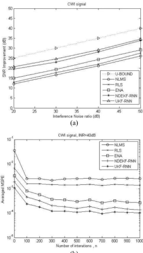
(a) CWI signal: Figure 3 presents the SNR improve-ments and averaged MSPE for single-tone CWIs. The continuous wave interference considered here is a single-tone sinusoidal signal. The CWI offset frequency is set as

= 1.2 MHz,  is a random phase uniformly distributed over the interval [0, 2), and the interference noise ratio (INR) is varied from 20 dB to 50 dB. The UKF-RNN algo-rithm can achieve faster convergence rates and better SNR improvement values than the other algorithms. On average, the UKF-RNN method provides 1.14 dB, 5.29 dB, 7.20 dB and 8.25 dB more in terms of SNR improvements than the NDEKF-RNN, ENA, RLS, and LMS methods, respec-tively. In Fig. 3(b), we compare the performance of the UKF-RNN algorithm with others by plotting the value of the MSPE versus the number of iterations. As we can see after about 300 iterations, the UKF-RNN has a better con-vergence rate than the LMS, RLS, ENA, and NDEKF-RNN. Figure 3(b) shows that the UKF-RNN scheme is also superior in both convergence speed and prediction error. The MSPE can decline significantly to 10–4 in 300 itera-tions, while the NLMS and RLS methods reach the steady state after 200 iterations and have larger MSPE results.

(a)

(b)

Fig. 3. Single tone CWI suppression performances of (a) SNR improvement vs. INR, (b) averaged MSPE vs. the number of iterations.

(a)

(b)

Fig. 4. Multiple tone CWI suppression performances of (a) SNR improvement vs. INR, (b) averaged MSPE vs. the number of iterations.

(b) Multi-tone CWI: The interfering signal considered is a five-tone signal, where the five offset frequencies are kept constant at i = 0.2 MHz, 0.4 MHz, 0.6 MHz,

0.8 MHz and 1 MHz, and i’s are i.i.d. random phases

uniformly distributed over the interval [0, 2). It is shown that UKF-RNN method has better convergence rates than all the other algorithms, and it can move rapidly to the steady state at about 300 iterations. As can be seen from Fig. 4(a) and (b), the simulation results are similar to those in the case of the CWI signal. On average, the UKF-RNN method offers 1.94 dB, 5.48 dB, 7.22 dB and 8.66 dB more in terms of SNR improvements than NDEKF-RNN, ENA, RLS, and LMS methods, respectively.

(2) Nonstationary jamming signals

(a)

(b)

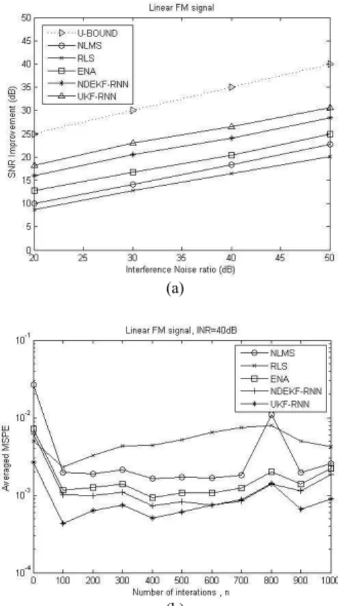
Fig. 5. Linear FM suppression performances of (a) SNR

improvement vs. INR, (b) averaged MSPE vs. the number of iterations.

(a)

(b)

Fig. 6. Pulsed tone CWI suppression performances of (a) SNR improvement vs. INR, (b) averaged MSPE vs. the number of iterations.

interval. In each simulation, the change in frequency hap-pens at the 750th iteration point, so a transient state is pre-sented in each curve. For the RLS algorithm, it is shown that that it performs poorly at estimating nonstationary signals. The step size of the LMS filter is constant, so the rate of convergence is limited. The performance of the LMS-based ENA filter is between those of the LMS/RLS and NDEKF-RNN filters. Because the Kalman gain matrix of the NDEKF-RNN and UKF-RNN methods allows an adjustable learning rate, we can see that it achieves a faster convergence rate in the transient state.

(b) Pulsed CWI: Another nonstationary signal we considered is the pulsed CWI. In this experiment, the frequency offset is set to 0.5 MHz, the on-interval is set at 1000 Tc and the off-interval is set at 500 Tc. Simulation

results of SNR improvements are given in Fig. 6(a). It is shown that the UKF-RNN method provides superior SNR improvements on both on- and off-intervals. On average, the UKF-RNN method offers 2.39 dB, 5.52 dB, 7.52 dB and 9.47 dB more in the SNR improvements than the NDEKF-RNN, ENA, RLS, and LMS methods, respec-tively. In Fig. 6(b), the off-interval is from the 500th to the 1000th iteration points, and others are on-interval. It is shown that the convergence speed of the MSPE of the UKF-RNN is usually faster than those of the LMS, RLS, ENA and NDEKF-RNN algorithms in both the on- and off-intervals.

5.

Conclusions

Radio frequency interference is one of the foremost concerns in safety and positioning critical applications that utilize GNSS receivers. A recurrent neural network using an UKF algorithm has been proposed to suppress GPS narrowband interference. The UKF-RNN method, which is an improved derivative-free and powerful nonlinear esti-mation approach, can robustly estimate the stationary and nonstationary jamming signals. The proposed RNN filter converges fast and guarantees its robustness against differ-ent kinds of obstacles. The UKF recursions are conducted and the corresponding cancellation performances are pre-sented. Simulation results have also confirmed that the proposed UKF-RNN algorithm improves the capability of combating interference and of accelerating the convergence rate. The results illustrate that the UKF-based RNN method is capable of increasing the SNR improvement and reduc-ing the MSPE of the received signals over those of the conventional methods in various interference circum-stances.

Acknowledgments

References

[1] KAPLAN, E. D., HEGARTY, C. J. Understanding GPS:

Principles and Applications. 2nd _{ed., rev. London (UK): Artech}

House, 2006. ISBN: 9781580538947

[2] DOVIS, F., MUSUMECI, L., LINTY, N., PINI, M. Recenttrends in interference mitigation and spoofing detection. International Journal of Embedded and Real-Time Communication Systems,

2012, vol. 3, p. 1–17. DOI: 10.4018/jertcs.2012070101

[3] LI, L. M., MISTEIN, L. B. Rejection of pulsed CW interference in PN spread spectrum systems using complex adaptive filter. IEEE

Transactions on Communications, 1983, vol. 31, no. 1, p. 10–20.

DOI: 10.1109/TCOM.1983.1095722

[4] RUSCH, L. A., POOR, H. V. Narrowband interference suppression in CDMA spread spectrum communications. IEEE

Transactions on Communications, 1994, vol. 42, no. 2-3-4,

p. 1969–1979. DOI: 10.1109/TCOMM.1994.583411

[5] GLISIC, S. G., MAMMELA, A., KAASILA, V. P., PAJKOVIC, M. K. Rejection of frequency sweeping signal in DS spread spectrum systems using complex adaptive filters. IEEE

Transactions on Communications, 1995, vol. 43, no. 1, p. 136–145.

DOI: 10.1109/26.385934

[6] CHANG, P. R., HU, J. T. Narrow-band interference suppression in spread spectrum CDMA communications using pipelined recurrent neural network. IEEE Transactions on Vehicular Technology. 1999, vol. 48, no. 2, p. 467–477. DOI: 10.1109/25.752570

[7] WILLIAMS, R. J., ZIPSER, D. A learning algorithm for continually running fully recurrent neural networks. Neural

Computation, 1989, vol. 1, p. 270–280. ISSN: 0899-7667. DOI:

10.1162/neco.1989.1.2.270

[8] CONNOR, J. T., MARTIN, R. D., ATLAS, L. E. Recurrent neural networks and robust time series prediction, IEEE Transactions on

Neural Network, 1994, vol. 5, no. 2, p. 240–254. DOI:

10.1109/72.279188

[9] JULIER, S. J., UHLMANN, J. K. Unscented filtering and nonlinear estimation. Proceedings of the IEEE, 2004, vol. 92, no. 3, p. 401–422. DOI: 10.1109/JPROC.2003.823141

[10] WU, X. WANG, Y. Extended and unscented Kalman filtering based feedforward neural networks for time series prediction.

Applied Mathematical Modelling, 2012, vol. 36, no. 3, p. 1123–

1131. DOI: 10.1016/j.apm.2011.07.052

[11] CHIEN, Y. R. Design of GPS anti-jamming systems using adaptive notch filters. IEEE System Journal, 2015, vol. 9, no. 2, p. 451–460. DOI: 10.1109/JSYST.2013.2283753

[12] CAPOZZA, P. T., HOLLAND, B. J., HOPKINSON, T. M., LANDRAU, R. L. A single-chip narrow-band frequency-domain excisor for a Global Positioning System (GPS) receiver. IEEE

Journal of Solid-State Circuits, 2000, vol. 35, no. 3, p. 401–411.

DOI: 10.1109/4.826823

[13] SAVASTA, S., LO PRESTI, L., RAO, M. Interference mitigation in GNSS receivers by a time-frequency approach. IEEE

Transactions on Aerospace and Electronic Systems, 2013, vol. 49,

no. 1, p. 415–438. DOI: 10.1109/TAES.2013.6404112

[14] SURENDRAN K. SHANMUGAM. Narrowband interference suppression performance of multi-correlation differential detection.

In Proceedings of ENC-GNSS 2007. Geneva (Switzerland), May

29-31, 2007, p. 1–12.

[15] QIANG, W., ZHANG, J., JING, Y. Nonlinear adaptive joint filter for narrowband interference suppression in GPS receiver. In 5th International Conference on Computer Sciences and Convergence

Information Technology (ICCIT). Seoul (Korea), 2010, p. 400–404.

ISBN: 978-1-4244-8567-3. DOI: 10.1109/ICCIT.2010.5711091

About the Author ...