(Annals of the Brazilian Academy of Sciences) ISSN 0001-3765
www.scielo.br/aabc
Multiphysical modelling of fluid transport through osteo-articular media
THIBAULT LEMAIRE, SALAH NAILI and VITTORIO SANSALONE
Laboratoire de Modélisation et Simulation Multi-Echelle, Biomécanique, CNRS 3160 MSME, Université Paris Est, 61, Avenue du Général de Gaulle, 94010 Créteil Cédex, France
Manuscript received on June 6, 2008; accepted for publication on November 5, 2008
ABSTRACT
In this study, a multiphysical description of fluid transport through osteo-articular porous media is pre-sented. Adapted from the model of Moyne and Murad, which is intended to describe clayey materials behaviour, this multiscale modelling allows for the derivation of the macroscopic response of the tissue from microscopical information. First the model is described. At the pore scale, electrohydrodynamics equations governing the electrolyte movement are coupled with local electrostatics (Gauss-Poisson equa-tion), and ionic transport equations. Using a change of variables and an asymptotic expansion method, the macroscopic description is carried out. Results of this model are used to show the importance of couplings effects on the mechanotransduction of compact bone remodelling.
Key words: biomechanics, multi-scale, homogenization, osteo-articular tissues, coupling effects.
1 INTRODUCTION
Osteo-articular media, such as bone tissues or cartilage, are complex saturated porous tissues composed of a solid matrix, cells and a fluid phase. The movement of the fluid phase within the spaces of the solid matrix is referred to as interstitial fluid flow. Although much is suspected about the role of fluid movement on biological activities such as growth, adaptation and repair mechanisms, relatively little is known about flow
characteristics underin vivoconditions. The behaviour of osteo-articular tissue is governed by different
effects due to many driving forces (hydraulic, biochemical, electrical, mechanical, etc.). For instance, the measurements of streaming potentials are commonly used to validate poroelastic models of bone (Salzstein et al. 1987, Salzstein and Pollack 1987, Cowin et al. 1995). In parallel, the role of electro-chemical phenomena in tissue remodelling and growth has been put into relief (Frank and Grodzinsky 1987a, b, Pollack 2001, Knothe Tate 2003, Sharma et al. 2007, Lemaire et al. 2008).
In this study, a multiphysical description of fluid transport through compact bone tissue is presented.
Thanks to this modelling, it is possible to estimate thein vivoelectro-chemical part of the fluid stimulation
Selected paper presented at the IUTAM Symposium on Swelling and Shrinking of Porous Materials: From Colloid Science to Poromechanics – August 06-10 2007, LNCC/MCT.
of the cells. Our approach is based on several previous works carried out under the aegis of Moyne and Murad (2002, 2006, Murad and Moyne 2006, 2008) and Lemaire et al. (2002, 2007, Lemaire 2004). All of these works aim at studying the hydro-mechanical behaviour of expansive clayey materials. Since the solid-fluid interface of these media presents a negative surface charge, many electro-physical phenomena, such as osmotic swelling, streaming potentials or electro-osmosis, may occur. Osteo-articular tissues present the same kind of electrical property. Indeed, bone matrix and cell membranes present negative surface potentials because of the presence of fatty acids and adsorbed species. In this paper, we intend to use the approach of Moyne and Murad to study interstitial fluid velocities in compact bone as it was done a few years ago (Lemaire et al. 2006). Nevertheless, we recently pointed out the necessity to improve the microscopical description of the living tissue (Lemaire et al. 2008) and proposed to add a parameter to describe the influence of a sub-microscopical structure corresponding to the fiber matrix surrounding the cells.
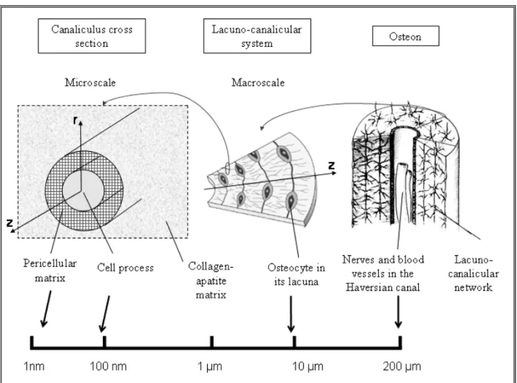
First the model is carried out. The two-scale saturated porous medium is composed by fluid and solid phases. This solid phase includes the cells and the bone matrix, whereas the fluid phase corresponds to the interstitial fluids. Typically, in compact bone, the microscale refers to the size of the micropores (the
canaliculi, whose radius is∼10−8m), whereas the macroscale corresponds to the osteon radius (10−4m).
The multiscale structure of compact bone is detailed in Section 4.1.
At the pore scale, electro-hydrodynamics equations governing the electrolyte movement are coupled with local electrostatics (Gauss-Poisson equation) and ionic transport equations. In particular, the fluid movement at the microscale is described thanks to a Brinkman equation. Indeed, in living tissues, the micropores that contain the cells are partially filled by a pericellular fibrous network. This network generates supplementary viscous effects. Thus, since a classical Stokesian approach cannot take into account this
sub-microscopical friction effect, a Brinkman-like term is added thanks to a permeability parameter Kf.
Using the change of variables proposed by Moyne and Murad (2002) and an asymptotic expansion method (Auriault 1991b), a macroscopic description of the fluid flow is derived.
The efficiency of this model is, then, presented in a biological application dealing with the mechan-otransduction of bone remodelling. Indeed, after having briefly introduced the multi-scale structure of compact bone, the key role of interstitial fluid movements in the vicinity of the mechano-sensitive cells of bone is discussed, and the importance of osmotic and electro-osmotic coupled phenomena at this scale is clearly demonstrated.
2 MICROSCOPICAL EQUATIONS IN THE FLUID PHASE
the approach, the chemical exchanges among the different phases of the medium are not taken into account. Hence, the surface charge of the medium remains constant. In what follows, we begin by presenting the microscopic phenomena that govern electric potential distribution, ion transport and fluid flow.
2.1 ELECTROSTATICS
Neglecting magnetic effects, the electric potentialφ in the fluid satisfies the Gauss-Poisson equation:
∇ ∙ ∇φ = − F
εε0
(n+−n−), (1)
where∇∙ is the divergence operator, ∇ the gradient operator, F the Faraday’s constant, ε0 the vacuum
permittivity,εthe relative dielectric constant of the solvent, and,n+andn−the cationic and anionic molar
concentrations, respectively.
Boundary conditions are obtained by writing the electric flux continuity at the pore’s walls. Notingσ
the surface charge density andnthe normal unit vector exterior to the the fluid domain, we have:
∇φ∙n= σ
εε0
. (2)
2.2 IONSTRANSPORT
The convection-diffusion equations of Nernst-Planck that governs the ion transport are:
∂n±
∂t + ∇ ∙(n
±v)= ∇ ∙
D±(∇n±±n±∇ ˉφ)
, (3)
wheretis the time,D+andD−are the water-ions diffusion coefficients for cations and anions, respectively.
The vectorvis the fluid velocity. The reduced electric potentialφˉ = Fφ/RT is introduced with the help
of absolute temperatureT and ideal gas constant R.
Boundary conditions are written considering the impervious property of the pore’s walls. Notingnthe
normal unit vector exterior to the the fluid domain, we have:
−D± ∇n±±n±∇ ˉφ
∙n=0. (4)
2.3 MODIFIEDBRINKMANEQUATION
of this supplementary damping force. Following the arguments of Brinkman (1947), a dissipative new term is added to the modified Stokes equation:
−∇p+μf∇ ∙ ∇v−
μf
Kf
v=F(n+−n−)∇φ, (5)
where p is the hydraulic pressure,μf is the fluid dynamic viscosity and Kf is an intrinsic permeability
parameter quantifying the damping effect due to the fibrous matrix.
Although the Brinkman equation is semi-empirical in nature, it has been validated by detailed numerical tests of the Stokes equation in regions near the interface among dissimilar regions (Martys et al. 1994).
Furthermore mass conservation equation is written as:
∇ ∙v=0. (6)
Boundary conditions at the interface are no-slip conditions:
v=0. (7)
2.4 ANALTERNATIVEFORMULATION IN THEFLUIDPHASE
An original approach of this multiphysical treatment of interstitial fluid flow within charged porous media consists in introducing a change of variables to separate microscopic variables that may vary at the pore’s scale, and macroscopic variables that only vary at the macroscopic scale. This change of variables is detailed elsewhere (Moyne and Murad 2003, Lemaire et al. 2002, 2006). Its principle consists in building at each
location of the fluid phase an equivalent virtual bulk (bulk’s fields are indexedb) which is at thermodynamical
equilibrium (in terms of electro-chemical potentialsμ), and conserves the electro-neutrality condition:
μ±b = μ± = ±Fφ+RTln(n±)= ±Fψb+RTln(n±b), (8)
n+b = n−b =nb. (9)
Consequently, bulk’s and real fields are linked as follows:
φ = ψb+ϕ, (10)
n± = nbexp(∓ ˉϕ), (11)
pb = p−π = p−2RT nb(coshϕˉ−1), (12)
whereπ is Donnan osmotic pressure.
The electric potential is, thus, decomposed into a bulk electric potential ψbplaying a similar role as
the streaming potential, and another potentialϕcorresponding to the double-layer potential (see Eq. (10)).
When the quantityϕis reduced toϕˉ = Fϕ/RT, this later potential rules the Boltzmann distributions of the
ionic species given by (11). The bulk concentration, which verifies the electro-neutrality condition (9), also appears in these ionic distributions. Finally, the bulk pressure can be expressed by subtracting the Donnan
As a consequence, the problem can be reformulated in terms of bulk variables. Equation (1) is rephrased to obtain the Poisson-Boltzmann equation:
∇ ∙ ∇(ψˉb+ ˉϕ)=
1
L2D sinhϕ,ˉ (13)
where the streaming potential has been reducedψˉb= Fψb/RT.
The Debye length LD =
p
εε0RT/(2F2nb), which characterizes the thickness of the diffuse double
layers, is here introduced. Furthermore, the new form of the Nernst-Planck equation (3) is:
∂
∂t nbexp(∓ ˉϕ)
+ ∇ ∙ nbexp(∓ ˉϕ)v
= ∇ ∙ D±exp(∓ ˉϕ)(∇nb±nb∇ ˉψb)
. (14)
Finally, the modified Brinkman equation (5) is reformulated:
μf∇ ∙ ∇v−
μf
Kf
v− ∇pb−2RT(coshϕˉ−1)∇nb+2RT nbsinhϕˉ ∇ ˉψb=0. (15)
In this expression, the different terms governing the fluid transport can be identified: i) the effect of the viscous shearing stresses acting on a volume element of fluid; ii) the effect of the damping force of the fibrous matrix; iii) the hydraulic driving effect due to the gradient of bulk pressure; iv) the osmotic driving effect due to the gradient of bulk concentration; v) the electro-osmotic driving effect due to the gradient of bulk electric potential. We can notice that the change of variables does not change the mass conservation equation (6).
The boundary conditions (2) and (4) are finally reformulated in terms of bulk variables:
∇(ψˉb+ ˉϕ)∙n =
Fσ εε0RT
, (16)
−D±exp(∓ ˉϕ)(∇nb±nb∇ ˉψb)∙n = 0. (17)
No-slip conditions for the velocity (7) are not modified by the change of variables.
3 HOMOGENIZATION PROCEDURE
The aim of this section is to propagate the microscopic phenomena presented in term of bulk variables to the upper scale. This change of scale is carried out within the general framework of periodic homogenization (Auriault 1991a). Thus, the bounded macroscopic medium is assumed to be made by a repeated microscopic
cell. The microscopic lengthℓcharacterizing the cell defines the length-scale for which the microscopic
heterogeneities are relevant. At the macroscopic length-scaleLof the porous medium, these heterogeneities
are no more significant. The ratio η = ℓ/L corresponds to the perturbation parameter. To obtain a
macroscopic equivalent description, the influence of the inhomogeneities of the microscopic scale has to
decay asymptotically as the ratioη decreases. As a consequence, this ratio has to be very small when
compared with one.
3.1 NON-DIMENSIONALWRITING OF THEMICROSCOPICPROBLEM
The first step of the periodic homogenization procedure consists in writing the microscopic equations in a
the microscale by reference values:
q′= q
qr
. (18)
The subscript “r” and the prime are respectively assigned to the reference values that are used to
normalize each quantity and to the resulting non-dimensional quantity. For instance, the reference length
Lr is chosen to be on the order of the macroscopic medium length, i.e., Lr ≡ L. In compact bone,
this macroscopic length corresponds typically to the osteon radius (10−4 m). This reference length is
used to obtain the non-dimensional writing of spatial derivative operators. Moreover, the reference values corresponding to constant quantities are these quantities themselves.
3.1.1 Micro/macro coordinates and spatial operator
Microscopic and macroscopic coordinatesxandXrespectively associated with the microscopic cell and the
overall dimension of the medium are introduced. The associated reference lengths are xr ≡ℓandXr ≡L
(Lemaire et al. 2006). As a consequence, choosing the reference characteristic length Lr on the order of
the macroscopic medium length, i.e. Lr ≡L, the spatial differential operator∇is transformed as:
∇ = 1
L∇
′= 1
ℓ∇
′
x +
1
L∇
′
X, (19)
where∇x and∇X are the differential operators referring to the microscopic and macroscopic coordinates,
respectively. Thus, we have finally:
∇′ =η−1∇x′ + ∇′X. (20)
3.1.2 Poisson-Boltzmann equation
To transform Eq. (13), the chosen reference electric potentialφr corresponds to the surface potential of the
pore walls. For instance, in bone tissues, this electric potential can be approximated by the values of the
zeta potential measured in bone tissue by Berreta and Pollack (1986): φr = −3.55 mV. As a consequence,
the non-dimensional number representing the reduced reference potential φˉr = Q = Fφr/RT is scaled
toO(η0), whereO()is big-oh notation that is used to describe the asymptotic behaviour of the function.
This implies thatψˉ′
b≡ ˉψbandϕˉ′ ≡ ˉϕ.
Moreover, the bulk concentration plays a role in the definition of the Debye length. It is, then, necessary to propose a reference value for this concentration. Following Moyne and Murad’s arguments (Moyne and
Murad 2002), local electroneutrality leads to a 1/ℓfaster variation of the ionic concentrations, in comparison
with the changes of the pore’s surface charge density σ. Thus, these authors proposed to express the
reference concentration asnr ≡σ/Fℓ. Moreover, the condition of electrical flux continuity at the interface
provides thatσ ≡εε0φr/ℓand reference concentration is rewritten asnr ≡εε0φr/Fℓ2. According to these
scaling laws, we haveLDr ≡ℓ. As a consequence, the Poisson-Boltzmann Eq. (13) is rephrased in:
η2∇′∙ ∇′(ψˉb′ + ˉϕ′)= 1
L′2D sinhϕˉ
′. (21)
Furthermore, the electrical flux continuity condition (16) is transformed in:
Using local electro-neutrality, this number can be interpreted as the ratio between the electrical and thermal
energiesQ= Fσ ℓ/εε0RT.
3.1.3 Nernst-Planck equations
The temporal differential-operator is scaled thanks to the reference time tr = L2/Dr, where Dr =
max(D+,D−)and max is the function that returns the maximum value. Thus, the Nernst-Planck Eq. (14)
is rewritten as:
∂ ∂t′ n
′
bexp(∓ ˉϕ′)
+Pe∇′∙ n′bexp(∓ ˉϕ′)v′
= ∇′∙ D′±exp(∓ ˉϕ′) ∇′n′b±n′b∇′ψˉb
′
), (23)
where the Péclet number is defined byPe =vrL/Dr. The quantity vr is a reference velocity.
Different cases can be viewed depending on the nature of the main driving effect (Auriault and Adler
1995). If diffusion is predominant, the Péclet number is small Pe= O(η). If convection at the large scale
is predominant, the Péclet number is important Pe = O(η−1). Finally, if convection and diffusion are
equivalent, we havePe =O(1).
The impervious condition (17) is also rephrased:
−D′
±exp(∓ ˉϕ ′)(∇n′
b±n′b∇ ˉψb
′
)∙n=0. (24)
3.1.4 Modified Brinkman equation
We introduce the Reynolds number Re = prL/μfvr and the number De = RT nr/pr, which measures
the importance of the osmotic effects related to the pressure effects. The intrinsic permeability Kf, which
quantifies the friction effect generated by the fibers, has to be reduced by a squared length. The order of magnitude of this permeability can be calculated thanks to the model of Tsay and Weinbaum (1991) adapted by Weinbaum et al. (1994). Thus, physiologically significant values of this parameter lay between
5.9 ×10⁻¹⁸ m2 and 2.0 ×10⁻¹⁷ m2 (Lemaire et al. 2008). Consequently, we choose to reduce the
permeability parameter with the squared microscopic lengthℓ2. The modified Brinkman equation is, then,
rewritten in its non-dimensional form: 1
Re
μ′f∇′∙ ∇′v′− 1
η2Re
μ′f
K′fv
′ = ∇′p′
b+De2R′T′(coshϕˉ′−1)∇′n′b−De2R′T′n′bsinhϕˉ
′∇′ψˉ′
b. (25)
Moreover, the mass conservation equation (6) is written in its non-dimensional form:
∇′∙v′ =0. (26)
Finally, the no-slip condition (7) at the solid-fluid interface is rephrased:
v′ =0. (27)
3.2 ASYMPTOTICEXPANSIONS
Each quantityq is expressed as a function depending on both the scales q = q(x,X). Moreover, it is
written in terms of asymptotic expansion of the small parameterη:
q(x,X)=
∞ X
i=0
For constant quantities, we can notice thatq[i](x,X) = 0 fori > 0 and, thus,q(x,X) = q[0] = q. These asymptotic expansions are introduced in the previous equations. Using the decomposition of the
spatial derivative operator (see Eq. (20)) in the previous equations, we collect the different powers ofη.
3.2.1 Developments of the Boltzmann terms
Combining the asymptotic expansion of the double-layer potential ϕˉ′ = ˉϕ[0]′ + ˉϕ[1]′ η+ ˉϕ[2]′ η2+ O(η3)
with a Taylor development at the origin of the exponential function, the Boltzmann term exp(∓ ˉϕ) is
expanded at the second order:
exp(∓ ˉϕ′)=exp(∓ ˉϕ[0]′ ) 1∓ ˉϕ′[1]η+ ϕˉ
′2 [1]
2 ∓ ˉϕ
′ [2]
η2+O(η3). (29)
Hence, the expansions of hyperbolic cosine and sine functions at the first order are, respectively:
cosh(ϕˉ′) = cosh(ϕˉ[0]′ )+ ˉϕ[1]′ sinh(ϕˉ[0]′ )η+O(η2) , (30)
sinh(ϕˉ′) = sinh(ϕˉ[0]′ )+ ˉϕ′[1]cosh(ϕˉ[0]′ )η+O(η2) . (31)
3.2.2 Poisson-Boltzmann equation
At the zeroth order, the Poisson-Boltzmann equation gives:
∇x′ ∙ ∇x′ϕˉ[0]′ + ∇′xψˉb′
[0]
= 1
L′D[0]
1
L′D[0] sinhϕˉ
′
[0]. (32)
The corresponding boundary condition at the zeroth order is obtained from the equation (22):
∇x′ ψˉb′
[0]+ ˉϕ ′ [0]
∙n= Q. (33)
3.2.3 Nernst-Planck equation
To study the Nernst-Planck equations, the Péclet’s number has to be scaled in regards to the transport process. For the case of transport within cortical bone’s lacuno-canalicular system, the reference length corresponds to the osteon’s radius and typical values of velocities have been calculated by Rémond et al. (2008). Comparing to the order of magnitude of classical diffusion coefficients in water, the main part of
ionic transport is diffusive and the Péclet’s number is small. Thus,Pe =O(η)and the asymptotic expansion
of the Nernst-Planck equation is carried out. Collecting the terms at the second order, we have:
∇x′ ∙
D±′ exp(∓ ˉϕ[0]′ ) ∇x′n′b
[0]±nb[′0]∇ ′
xψˉ
′
b[0]
=0. (34)
At the first order, we obtain:
∇′X∙
D±′ exp(∓ ˉϕ[0]′ ) ∇′xn′b
[0]±n ′
b[0]∇ ′
xψˉ
′
b[0]
+ ∇x′ ∙
D±′ exp(∓ ˉϕ[0]′ ) ∇X′n′b
[0]
+∇x′n′b
[1]±n ′
b[0] ∇ ′
Xψˉ
′
b[0]+ ∇ ′
xψˉ
′
b[1]
±n′b
[1]∇ ′
xψˉ
′
b[0]∓ ˉϕ ′ [1]∇x′n
′
b[0]− ˉϕ ′ [1]n′b[0]∇
′
xψˉ
′
b[0]
Finally, the ionic transport gives at the zeroth order:
∂ ∂t(n
′
b[0]exp(∓ ˉϕ ′
[0]))+ ∇x′ ∙(n
′
b[0]exp(∓ ˉϕ ′
[0])v′[0])=
∇′X∙(D′±exp(∓ ˉϕ′[0])(∇′Xn′b[0]+ ∇ ′
xn′b[1]∓ ˉϕ ′
[1]∇x′n′b[0]))+ ∇ ′
x ∙(D±′ exp(∓ ˉϕ ′
[0])(∇X′n′b[1] + ∇ ′
xn′b[2]))
∓ ∇x′ ∙(D±′ exp(∓ ˉϕ[0]′ )ϕˉ[1]′ (∇′Xn′b[0]+ ∇ ′
xn′b[1]))+ ∇ ′
x ∙(D±′ exp(∓ ˉϕ ′ [0])(
ˉ
ϕ[1]′
2 ∓ ˉϕ
′
[2])∇x′n′b[0])
± ∇′X∙(D±′ exp(∓ ˉϕ′[0])n′b[0](∇′Xψˉb′
[0] + ∇ ′
xψˉ
′
b[1]))± ∇ ′
x∙(D
′
±exp(∓ ˉϕ ′
[0])n′b[1](∇ ′
Xψˉ
′
b[0]+ ∇ ′
xψˉ
′
b[1]))
± ∇x′ ∙(D±′ exp(∓ ˉϕ[0]′ )n′b[0](∇X′ψˉb′
[1]+ ∇ ′
xψˉ
′
b[2]+(
ˉ
ϕ[1]′
2 ∓ ˉϕ
′ [2])∇x′ψˉ
′
b[0]))
± ∇′X∙(D±′ exp(∓ ˉϕ′[0])(n′b
[1]∓ ˉϕ ′
[1]n′b[0])∇ ′
xψˉ
′
b[0])± ∇ ′
x ∙(D
′
±exp(∓ ˉϕ ′
[0])n′b[2]∇ ′
xψˉ
′
b[0])
− ∇x′ ∙(D±′ exp(∓ ˉϕ[0]′ )ϕˉ[1]′ (n′b
[0](∇ ′
Xψˉ
′
b[0]+ ∇ ′
xψˉ
′
b[1])+n ′
b[1]∇ ′
xψˉ
′
b[0])).
(36)
Moreover, the impervious boundary condition (24) gives, respectively, at the first and zeroth orders:
−D±′ exp(∓ ˉϕ′[0])(∇x′n′b[0]±n ′
b[0]∇ ′
xψˉb′[0])∙n=0, (37)
−D±′ exp(∓ ˉϕ[0]′ )[∇′Xn′b
[0]+ ∇ ′
xn
′
b[1]±n ′
b[0](∇ ′
Xψˉ
′
b[0]+ ∇ ′
xψˉ
′
b[1])±n ′
b[1]∇ ′
xψˉb[0]
∓ ˉϕ′[1](∇′xn′b[0] ±n ′
b[0]∇ ′
xψˉb′[0])] ∙n=0. (38)
3.2.4 Brinkman equation
Two non-dimensional numbers have been introduced in the Brinkman equation (25). It is, then, necessary
to estimate their order of magnitude. On the one hand, the Reynolds number Re = prL/μfvr, which
compares inertial and viscous effects, is quantified using the scaling law proposed by Auriault (1991a).
The orders of magnitude of the reference velocity vr and pressure pr of the fluid are based on classical
dimensional analysis of Darcy law, which leads to vr ≡ℓ2pr/μfL. Consequently, we have the order of
magnitude of the Reynolds numberRe ≡O(η−2). On the other hand, according to Derjaguin et al. (1987),
electrical stresses counterbalance the osmotic pressure effects. This argument leads to an estimation of the
non-dimensional numberDe. Indeed, since electrical and pressure effects have the same order of magnitude,
we haveDe≡ O(1). Using these scaling laws in the Brinkman problem, the collection of terms at the first
and zeroth orders gives:
0= ∇x′p′b
[0]+2R
′T′ cosh
ˉ
ϕ[0]′ −1∇x′n′b
[0]−2R ′T′n′
b[0]sinhϕˉ ′ [0]∇x′ψˉ
′
b[0], (39)
μ′f∇x′ ∙ ∇x′v′[0]− μ
′
f
K′
f
v′[0]= ∇′Xp′b
[0]+ ∇ ′
xp
′
b[1]+2R
′T′ cosh
ˉ
ϕ[0]′ −1 ∇′Xn′b
[0]+ ∇ ′
xn
′
b[1]
−2R′T′n′b
[0]sinhϕˉ ′ [0] ∇′Xψˉ
′
b[0] + ∇ ′
xψˉ
′
b[1]
−2R′T′n′b
[1]sinhϕˉ ′ [0]∇x′ψˉ
′
b[0]
+2R′T′ϕˉ[1]′ sinhϕˉ′[0]∇x′n′b
[0] −n ′
b[0]coshϕˉ ′ [0]∇x′ψˉ
′
b[0]
. (40)
at the first and zeroth orders:
∇x′ ∙v′[0] = 0, (41)
∇′X∙v′[0]+ ∇x′ ∙v[1]′ = 0. (42)
3.3 SLOWVARIABLES OF THEPROBLEM
The set of previous equations is used to separate variables that only vary at the macroscopic scale (slow variables) from those which possibly vary at the microscopic scale (fast variables).
For frequent geometries of pores such as parallel platelets (clayey materials, gels) or parallel cylindric channels (filters, bones, Kozeny-Carman materials), it is possible to make the cartesian or cylindric coor-dinates correspond to the macro and microscopic coorcoor-dinates. The example of the tubular geometry of the
canaliculiis used hereafter (see Section 4.1). When considering such a situation, the slow variables useful
for the model can be easily deduced. First, using the impervious condition (37) in equation (34), we show that the zeroth order terms of bulk concentration and potential do not vary at the microscopic scale. Taking into account this result in the first order of the Brinkman equation (39), we also obtain that the zeroth order term of the bulk pressure is a slow variable. Finally, bulk variables are only slow ones:
∇x′n′b
[0] = ∇ ′
xψˉ
′
b[0] = ∇ ′
xp
′
b[0] =0. (43)
This result shows the interest of working with bulk variables, since they only depend on the macroscopic coordinate.
To obtain this result for any geometry of the porous network, it is necessary to adopt another approach as proposed by Moyne and Murad (2002) to avoid the miscomprehension that appears by combining equations (34) and (37).
3.4 CONSEQUENCES ONPREVIOUSEQUATIONS
Considering that the slow variables do not vary at the microscale through equality (43), equations (32) to (40) can be simplified as follows:
∇x′ ∙ ∇x′ϕˉ[0]′ = 1
L′
D[0] 1
L′
D[0]
sinhϕˉ[0]′ , (44)
∇′xϕˉ′[0]∙n= Q, (45)
∇x′ ∙ D′±exp(∓ ˉϕ[0]′ ) ∇X′n′b
[0] + ∇ ′
xn
′
b[1]±n ′
b[0](∇ ′
Xψˉb[0]+ ∇ ′
xψˉb[1])
=0, (46)
∂ ∂t(n
′
b[0]exp(∓ ˉϕ ′
[0]))+ ∇x′ ∙(n
′
b[0]exp(∓ ˉϕ ′
[0])v′[0])=
∇X′ ∙(D±′ exp(∓ ˉϕ[0]′ )(∇X′n′b[0]+ ∇ ′
xn′b[1]))+ ∇ ′
x∙(D′±exp(∓ ˉϕ ′
[0])(∇′Xn′b[1]+ ∇ ′
xn′b[2]))
∓∇x′ ∙(D±′ exp(∓ ˉϕ[0]′ )ϕˉ[1]′ (∇′Xn′b[0]+ ∇x′nb′[1]))± ∇′X ∙(D±′ exp(∓ ˉϕ′[0])n′b[0](∇′Xψˉb′
[0] + ∇ ′
xψˉ
′
b[1]))
±∇x′ ∙(D±′ exp(∓ ˉϕ[0]′ )n′b
[1](∇ ′
Xψˉ
′
b[0]+ ∇ ′
xψˉ
′
b[1]))± ∇ ′
x∙(D
′
±exp(∓ ˉϕ ′
[0])n′b[0](∇ ′
Xψˉb[1]+ ∇ ′
xψˉ
′
b[2]))
−∇x′ ∙(D±′ exp(∓ ˉϕ[0]′ )ϕˉ[1]′ (n′b
[0](∇ ′
Xψˉ
′
b[0]+ ∇ ′
xψˉ
′
−D±′ exp(∓ ˉϕ[0]′ ) ∇′Xn′b[0]+ ∇ ′
xn′b[1]±n ′
b[0] ∇ ′
Xψˉb′[0]+ ∇ ′
xψˉb′[1]
∙n=0, (48)
μ′f∇x′ ∙ ∇x′v[0]′ − μ
′
f
K′fv
′
[0]= ∇′Xp
′
b[0]+ ∇ ′
xp
′
b[1]
+2R′T′ coshϕˉ[0]′ −1 ∇′Xn′b
[0]+ ∇ ′
xn
′
b[1]
−2R′T′n′b
[0]sinhϕˉ ′ [0] ∇X′ψˉ
′
b[0]+ ∇ ′
xψˉ
′
b[1]
. (49)
3.5 CLOSUREPROBLEMS
The next step consists in deriving the macroscopic description from the previous equations. If the Poisson-Boltzmann and the ionic transport equations can be treated similarly as proposed by Moyne and Murad (2002), the derivation of the macroscopic Darcy law is slightly different.
3.5.1 Local Poisson-Boltzmann equation
Because of the scaling factor in the Poisson-Boltzmann equation, this equation is purely expressed at the microscopical scale. If the Debye length is small compared to the pore size, this equation can, thus, be linearized thanks to the Debye-Hueckel approximation:
∇x′ ∙ ∇x′ϕˉ[0]′ = 1
L′D[0]
1
L′D[0]ϕˉ
′
[0]. (50)
3.5.2 Ionic transport
The macroscopic transport equations can be obtained by solving the closure problems of Nernst-Planck equations. To apply the homogenization procedure of the Taylor dispersion problem proposed by Auriault and Adler (1995), the change of variables proposed by Moyne and Murad (2002) is used to rephrase equations (46), (47) and (48). Indeed, to avoid working with the electro-migration term in the Nernst-Planck
model, these authors proposed to consider auxiliary concentrations n±f to recover classical
convection-diffusion equations, and suggested the following change of variables using the streaming potentialψthat
coincides with our bulk potentialψb:
n′±f =n′bexp(± ˉψ′) . (51)
The expansion of these auxiliary concentrations can be obtained from the development (29):
n′±f =
∞ X
i=0
n′f[i]ηi =n′b[0]exp(± ˉψ[0]′ )+exp(± ˉψ[0]′ ) n′b[1] ±n′b[0]ψˉ[1]′ η
+exp(± ˉψ[0]′ ) n′b[2]±n′b[1]ψˉ[1]′ +n′b[0]
ˉ
ψ[1]′2
2 ± ˉψ
′ [2]
η2+O(η3).
(52)
As a consequence, equation (46) becomes:
0= ∇x′ ∙(D±′ exp(∓ ˉϕ′[0]) ∇X′ n′f[0]+ ∇x′n′f[1], (53)
with the associated boundary condition derived from equation (48):
−D′±exp(∓ ˉϕ′[0]) ∇′Xn′f
[0]+ ∇ ′
xn
′
f[1]
These two last equations form the closure problem for n′
f[1] as obtained by Moyne and Murad (2002),
whose solution is presented by Auriault and Adler (1995).
Moreover, when rephrasing equation (47) in terms of fictitious concentrations and using the mass conservation equation (41), we have:
∂ ∂t n
′
f[0]exp(∓ ˉϕ ′ [0])
+v′[0]∙ ∇x′ n′f
[0]exp(∓ ˉϕ ′ [0])
= ∇X′ ∙D′±exp(∓ ˉφ′[0])(∇X′n′f
[0]+ ∇ ′
xn
′
f[1])
+∇′x∙D′±exp(∓ ˉφ[0]′ )(∇X′n′f
[1]+ ∇ ′
xn
′
f[2])∓ ˉφ ′ [1](∇′Xn
′
f[0]+ ∇ ′
xn
′
f[1])
.
(55)
Again, this equation is similar to the one treated by Moyne and Murad (2002) and can be rewritten as proposed by these authors.
3.5.3 Derivation of a macroscopic Darcy law
To rewrite the Brinkman equation (49), its linearity property is used. Thus, the fluid velocity is splitted into three terms: v′ =v′
P+v′C+v′E, wherev′P,v′Candv′Eare respectively associated with the Poiseuille, osmotic
and electro-osmotic flows. Brinkman equation is, then, decomposed into three independent equations with
similar no-slip conditions at thecanaliculuswall and cell membrane:
μ′f∇′x∙ ∇x′v′α[0]−
μ′f
K′
f
v′α[0] =F ′ α(∇
′
XG
′ α[0]+ ∇
′
xG
′
α[1]), (56)
where the subscript α = P,C or E stands respectively for the Poiseuille, osmotic and electro-osmotic
effects. The quantitiesGα andFα are expressed forα = P,C,Eby:
G′P = p′b, FP′ =1, (57)
G′C =n′b, FC′ =2R′T′(coshϕˉ[0]′ −1), (58)
G′E = ˉψb′, FE′ = −2R′T′n′b
[0]sinhϕˉ ′
[0]. (59)
Following the linearity arguments of Auriault and Adler (1995), the velocityv′
α[0]has the form:
v′α[0] = −κ ′ α∇
′
XG
′
α[0], for α = P,C,E, (60)
whereκ′
α is the second order tensor associated with the permeability at the pore’s scale corresponding to
theα driving gradient.
Introducing this expression ofv′α[0] into equation (56) yieldsG ′
α[1] in the form:
G′α
[1] = −β ′ α∙ ∇
′
XG
′ α[0] +g
′
α[1], for α= P,C,E, (61)
where g′
α[1] is an arbitrary function of the macroscopic variable X and β
′
α is an auxiliary ℓ-periodical
vector-valued function satisfying the cell problem:
∇x′β′α−μ
′
f
F′ α
∇x′ ∙ ∇x′κ′α+ μ
′ f F′ αK ′ f
κ′α −I=0, for α= P,C,E, (62)
Noting < . >the average over the representative unit cell, the seepage velocity due to theα driving
effect is given by:
<v′α[0] >= −K ′ α∇
′
XG
′
α[0], for α = P,C,E, (63)
where the second order permeability tensorK′
α =< κ′α >is introduced. Moreover, integrating over the
unit cell the continuity equation (42), we finally obtain the upscaled version of the Brinkman equation:
∇′X∙(K′α∇′XG′α
[0])=0, for α= P,C,E. (64)
Thus, for each of the three driving effects, equation (62) has to be solved to determine the permeability
Kα′. In parallel, the macroscopic flow can be determined from equation (64).
Hence, the averaged macroscopic fluid flow can be described through a modified Darcy law of the form:
<v[0]′ >=<v′P[0] >+<v ′
C[0] >+<v ′
E[0] >= −K ′
P∇′Xp′b[0]−K ′
C∇′Xn′b[0]−K ′
E∇′Xψˉb[0]. (65)
4 APPLICATION OF THE MODEL TO COMPACT BONE
In this section, we propose to illustrate the interest of this model in the scope of bone remodelling.
4.1 THESTRUCTURE OF COMPACTBONE
Compact bone presents a well organised structure composed of mineralized cylinders called osteons. These osteons, which are a few hundred micrometers in diameter, are centered on Haversian canals whose diameters
are on the order of 40−100μm (Cowin 2001). Osteons run primarily in the longitudinal axis of the bone.
These macrochannels contain the vasculature, the nerves and interstitial fluid.
Moreover, there are other extravascular pores in the solid matrix of the bone. For instance,lacunæare
ellipsoidal cavities with diameters of 10−30 μm occupied by osteocyte cells. Thecanaliculiare small
cylindric channels whose diameter is on the order of 0.1μm. They form a network connectinglacunæ
and the Haversian vascular canals. Cytoplasmic osteocyte cell process occupies the central zone of each
canaliculus, so that the interstitial fluid pathway corresponds to an annular geometry. As introduced in
Figure 1, thecanaliculus scale will be referred to as the microscale hereafter, whereas the macroscopic
length will correspond to the osteon. We introduce a cylindrical coordinate system to describe the geometry
of the annular space perfused by the fluid in thecanaliculi. The radial and longitudinal coordinatesr and
z are, thus, identified with the microscopic and macroscopic coordinates x and X, respectively. Since
canaliculi are mainly oriented in the radial direction of the osteon, the longitudinal coordinate z at the
canalicular scale corresponds to the radial direction at the osteon scale.
Furthermore, electron photomicrographs of the lacuno-canalicular system presented by You et al. (2004) showed the presence of nano-elements forming a fibrous pericellular matrix in the annular space of thecanaliculi. Even if this fibrous matrix obviously disturbs the interstitial fluid movement, its influence
on the tissue behaviour is not yet well understood. According to physiological arguments, Lemaire et
al. (2008) quantified its friction effect thanks to a very low permeability parameter Kf laying between
Fig. 1 – Multiscale structure of the cortical bone; the microscale corresponds to the radius of thecanaliculi, whereas the macroscale refers to the osteon radius.
4.2 DEBYE-HUECKELAPPROXIMATION
To solve the local electrical problem, the Debye-Hueckel approximation (see Eq. (50)) is used since the surface potential remains small (less than 25mV) and the pores are large enough in comparison with the Debye length. The analytical solution of this equation in a cylindrical geometry is given by Lemaire et al. (2006).
4.3 COUPLEDPERMEABILITYPARAMETERS AT THE PORESCALE
The coupled Darcy law is now derived in the context of compact bone. Considering that the fluid velocity
develops in the longitudinal direction of the pores and only depends on the canalicular radial coordinater,
we have three problems to solve, after projecting equation (56) onz-axis:
μf
d2uα
dr2 +
1
r duα
dr
− μf
Kf
uα =Fα
d Gα
d z , for α= P,C,E, (66)
whereuis the longitudinal component of the fluid velocity. From these equations, the permeability at the
pore scaleκα(r)can be calculated.
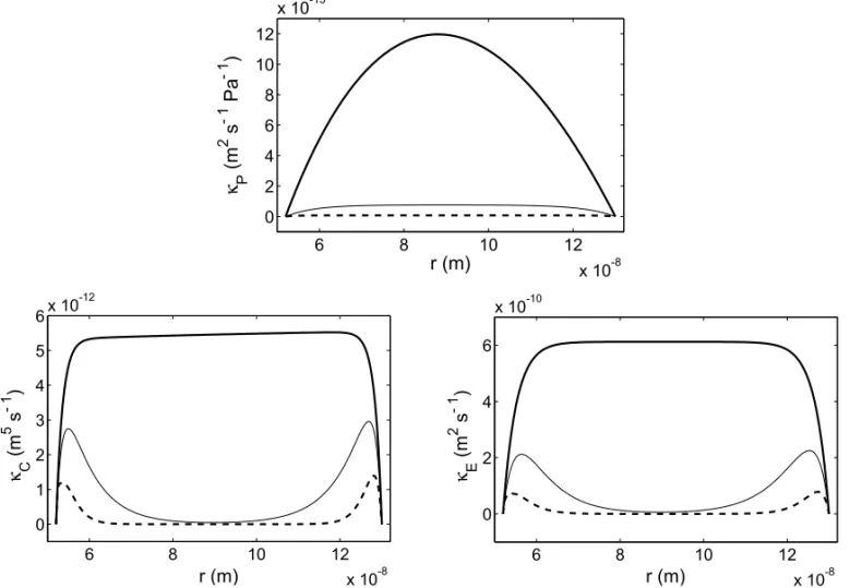
The spatial variation of the three velocities at the pore scale is shown in Figure 2 through plotting
these graphs are presented in Table I. To underline the effect of the fibers, the Stokesian case (Kf −→ ∞)
is also plotted.
6 8 10 12
x 10-8 0
2 4 6 8 10 12
x 10-13
r (m)
κ P
(m
2 s
-1 P
a
-1 )
6 8 10 12
x 10-8 0
1 2 3 4 5 6x 10
-12
r (m)
κ C
(m
5 s
-1 )
6 8 10 12
x 10-8 0
2 4 6
x 10-10
r (m)
κ E
(m
2 s
-1 )
Fig. 2 – Profile of the local permeability parametersκα, forα= P, C, E, at the pore’s scale considering Poiseuille effect (on the
top), Osmotic effect (on the left), Electro-osmotic effect (on the right) for various values of the fibers permeability parameterKf
expressed in m2:Kf −→ ∞(bold solid line),Kf =5×10⁻¹⁷(thin solid line),Kf =5×10⁻¹⁸(bold dashed line).
Quantitatively, the presence of the pericellular matrix does slow down the fluid flow. Within the realistic range of pericellular permeability values, the fluid velocity is scaled down by a factor of 1 000
(Kf = 5×10⁻¹⁸ m2) to 100 (Kf = 5×10⁻¹⁷ m2) in comparison with the one associated with a clear
fluid-filledcanaliculus.
Nevertheless, the decreases in velocity are not the same when comparing hydraulic and electro-chemical effects. Near the walls of the pore, the action of the negative double layer potential tends to maintain the electro-chemical effects. In the central zone, this electric potential action disappears and these effects are
less significant. In parallel, the hydraulic local permeabilityκP, which only depends on the geometry and
the fluid viscosity, is not affected by these local electric fluctuations.
4.4 CONSEQUENCES FOR THEMECHANOTRANSDUCTION
TABLE I
Parameters of the model. geometry
Canaliculus radius Rc=130 nm
Process radius Rm =52 nm
Osteon radius Lc=33μm
fluid parameters
Ionic concentration nb=0.01 M
Dielectric permittivity ε=75.34
Dynamic viscosity μf =0.65×10⁻³Pl
pore parameters
Surface potential φr = −20 mV
Pericellular permeability Kf ∈ [5×10−18,5×10−17]m2
macroscopic driving gradients (d Gα/d z)
Hydraulic effect (P) 10 000 Pa/Lc
Chemical effect (C) 0.05 M/Lc
Electric effect (E) 10 mV/Lc
coupled fluid shear stresses acting on the cell process membrane. Typically, thein vivoshear stress values
that initiate endothelial cell response are of a one or two Pascals. The order of magnitude of the shear stress calculated by Weinbaum et al. (1994) in cortical bone fits well with this value.
In order to evaluate this physical parameter, we approximate the macroscopic driving gradients thanks
to literature values of Table I. With our model, the shear effectτP generated by Poiseuille effect is similar
to the one generated by electro-osmosisτE(around 0.5 Pa) and is three times lower than the chemical shear
stressτC(around 1.5 Pa).
As a result, it is worth considering the coupled effects in the description of the fluid movement at the
canaliculusscale. It is all the more true when studying the mechanotransduction of bone remodelling.
CONCLUSION
Following the Moyne and Murad approach, a two-scale modelling of coupled phenomena governing
osteo-articular materials has been carried out. The difficulty to propose suitable in vivoexperimental studies
explains the strong need for sophisticated theoretical models that can describe the behaviour of living media. Through the results of our model, we propose a possible way to understand how the electro-chemical phenomena play a key role in the mechanotransduction of the bone remodelling. Contrary to classical models describing fluid flows in the bones, the coupled Darcy law developed in this study is able to quantify appreciable electrokinetics phenomena. This study has to be continued by introducing possible exchanges of ionic species between the fluid and cells to better describe cell activity.
ACKNOWLEDGMENTS
RESUMO
Neste estudo uma descrição multifísica do transporte de fluidos em meios porosos osteo articulares é apresentada. Adaptado a partir do modelo de Moyne e Murad proposto para descrever o comportamento de materiais argilosos a modelagem multiescala permite a derivação da resposta macroscópica do tecido a partir da informação microscópica. Na primeira parte o modelo é apresentado. Na escala do poro as equações da eletro-hidrodinâmica governantes do movimento dos eletrolitos são acopladas com a eletrostática local (equação de Gauss-Poisson) e as equações de transporte iônico. Usando uma mudança de variáveis e o método de expansão assintótica a derivação macroscópica é conduzida. Resultados do modelo proposto são usados para salientar a importância dos efeitos de acoplamento sobre a transdução mecânica da remodelagem de ossos compactados.
Palavras-chave:biomecânica, multiescala, homogeneização, tecidos osteo articulares, efeitos de acoplamento.
REFERENCES
AURIAULTJL. 1991a. Dynamic behaviour of porous media. In: BEARJANDCORAPCIOGLUMY (Eds), Transport
processes in Porous Media: Kluwer Academic Publishers. Appl Sci 202: 471–519.
AURIAULTJL. 1991b. Heterogeneous medium. Is an equivalent macroscopic description possible? Int J Eng Sci
29: 785–795.
AURIAULTJLANDADLERPM. 1995. Taylor dispersion in porous media: analysis by multiple scale expansions. Adv Water Resour 18: 217–226.
BERRETA DAND POLLACKS. 1986. Ion concentration effects on the zeta potential of bone. J Orthop Res 4:
337–341.
BRINKMANHC. 1947. A calculation of the viscous forces exerted by a flowing fluid on a dense swarm of particles. Appl Sci Res A1: 27–34.
BURGER EH, KLEIN-NULENDJAND SMIT TH. 2003, Strain-derived canalicular fluid flow regulates osteoclast
activity in a remodelling osteon-a proposal. J Biomech 36: 1453–1459.
COWINSC. 2001. Bone mechanics handbook, 2nded., CRC Press, Boca Raton, FL.
COWINSC, WEINBAUMSANDZENGY. 1995. A case for bonecanaliculias the anatomical site of strain generated
potentials. J Biomech 28: 1281–1297.
DERJAGUINB, CHURAEVNANDMULLERV. 1987. Surface forces, Plenum Press, New York.
FRANK EHAND GRODZINSKY AJ. 1987a. Cartilage electromechanics. I. Electrokinetic transduction and the
effects of electrolyte ph and ionic strength. J Biomech 20: 615–627.
FRANK EH AND GRODZINSKY AJ. 1987b. Cartilage electromechanics. II. A continuum model of cartilage
electrokinetics and correlation with experiments. J Biomech 20: 629–639.
GURURAJA S, KIM HJ, SWANCC, BRAND RA AND LAKES RS. 2005. Modeling deformation-induced fluid flow in cortical bone’s lacunar-canalicular system. Ann Biomed Eng 33: 7–25.
JACOBSCR, YELLOWLEYCE, DAVISBR, ZHOUZ, CIMBALAJMANDDONAHUEHJ. 1998. Differential effect
of steady versus oscillating flow on bone cells. J Biomech 31: 969–976.
KNOTHETATEML. 2003. “Whither flows the fluid in bone?” An osteocyte’s perspective. J Biomech 36: 1409–1424. LEMAIRE T. 2004. Couplages électro-chimio-hydro-mécaniques dans les milieux argileux, PhD thesis, Institut
LEMAIRET, MOYNEC, STEMMELENDANDMURADM. 2002. Electro-chemo-mechanical couplings in swelling clays derived by homogenization : electroviscous effects and onsager’s relations. In: AURIAULTJ, GEINDREAU
C, ROYERP, BLOCHJ-F, BOUTINCANDLEWANDOWSKAJ (Eds), ‘Poromechanics II’, Balkema Publishers,
Lisse, p. 489–500.
LEMAIRET, NAILISANDRÉMONDA. 2006. Multi-scale analysis of the coupled effects governing the movement of interstitial fluid in cortical bone. Biomechan Model Mechanobiol 5: 39–52.
LEMAIRE T, MOYNEC ANDSTEMMELEN D. 2007. Modelling of electro-osmosis in clayey materials including
ph effects. Phys Chem Earth 32: 441–452.
LEMAIRET, NAILIS ANDRÉMONDA. 2008. Study of the influence of fibrous pericellular matrix in the cortical
interstitial fluid movement. J Biomech Eng 130: 1–11.
MARTYS N, BENTZ D AND GARBOCZI E. 1994. Computer simulation study of the effective viscosity in Brinkman’s equation. Phys Fluids 6: 1434.
MOYNE C AND MURAD MA. 2002. Electro-chemo-mechanical couplings in swelling clays derived from a
micro/macro-homogenization procedure. Int J Sol Struct 39: 6159–6190.
MOYNEC ANDMURADMA. 2003. Macroscopic behavior of swelling porous media derived from micro-mechanical analysis. Transp Porous Med 50: 127–151.
MOYNECAND MURAD MA. 2006. A two-scale model for coupled electro-chemo-mechanical phenomena and
Onsager’s reciprocity relations in expasive clays: II computational validation. Transp Porous Med 63: 13–56. MURAD MA AND MOYNE C. 2006. Two-scale model for coupled electro-chemo-mechanical phenomena and
Onsager’s reciprocity relations in expansive clays: I homogenization analysis. Transp Porous Med 62: 333–380. MURADMAANDMOYNEC. 2008. A dual-porosity model for ionic solute transport in expansive clays. Comput
Geosci 12: 47–82.
POLLACKS. 2001. Streaming potentials in bone. In: COWIN S (Ed), Bone Mechanics Handbook, 2nded., CRC
Press, Boca Raton, FL.
RÉMOND A, NAILI S AND LEMAIRE T. 2008. Interstitial fluid flow in the osteon with spatial gradients of
mechanical properties: a finite element study. Biomech Modeling Mechanobiol 7: 487–495.
SALZSTEINRAANDPOLLACKSR. 1987. Electromechanical potentials in cortical bone. II. Experimental analysis.
J Biomech 20: 271–280.
SALZSTEINRA, POLLACKSR, MAKAFTANDPETROVN. 1987. Electromechanical potentials in cortical bone. I. A continuum approach. J Biomech 20: 261–270.
SHARMA U, MIKOS AGAND COWIN SC. 2007. Mechanosensory mechanisms in bone. In: Princ Tissue Eng,
Elsevier, p. 919–933.
TSAYR-YANDWEINBAUMS. 1991. Viscous flow in a channel with periodic cross-bridging fibers: exact solutions and brinkman approximation. J Fluid Mech 226: 125–148.
WEINBAUMS, COWINSCANDZENGY. 1994. A model for the excitation of osteocytes by mechanical
loading-induced bone fluid shear stresses. J Biomech 27: 339–360.