An axisymmetric nodal averaged finite element
Abstract
A nodal averaging technique which was earlier used for plane strain and three-dimensional problems is extended to include the axisymmetric one. Based on the virtual work principle, an expression for nodal force is found. In turn, a nodal force variation yields a stiffness matrix that proves to be non-symmetrical. But, cumbersome non-symmetrical terms can be rejected without the loss of Newton-Raphson iterations convergence. An approxi-mate formula of volume for a ring of triangular profile is exploited in order to simplify program codes and also to accelerate calculations. The proposed finite element is intended primarily for quasistatic problems and large irre-versible strain i.e. for metal forming analysis. As a test problem, deep rolling of a steel rod is studied.
Keywords
finite element, nodal averaging, axisymmetric problem, large strain, metal forming
1 INTRODUCTION
The finite element method (FEM) is widely used in science and engineering for numerical analysis of problems which beggar analytical methods. The specific character of solid mechanics tasks is that (except for porous media) a body shape can be varied greatly while body’s volume alters insignificantly. But, the approximating functions proposed by classical FEM (see for example the textbook Zienkiewicz (1971)) do not comply with the incompress-ibility requirement. At first sight, this does not induce any drawback because the convergence theorems have been proven for many FEM calculation schemes. Nevertheless, in practice (mainly when a personal computer is used) an approximate solution can be found to be too far from an exact one and such tasks were really discussed in last decades. This circumstance forced to revise all the classical approximations of tensor fields. Many new approaches have been developed but they require a special review. Plane strain, three-dimensional, and shell problems have been involved but the axisymmetric one remains out of consideration so far and the present work aim is elimination of this gap.
The first attempt to overcome the volumetric locking difficulties was the application of selective reduced inte-gration schemes to displacement-based nonlinear finite elements (bi-linear, tri-linear, second order, and third or-der). The deviatoric items of a variational equation are integrated by larger number of Gauss points P1,…,Pn while the volumetric items – by less number of points Q1,…,Qm (m<n). In general, it is impossible to meet the incompress-ibility requirements at all the points Pi but it is possible to do it at points Qi. This method suffers from many short-comings: sizable computer memory is needed to store the state parameters such as stress, strain, damage, etc. at Gauss points; problems appear when transferring data from one finite element mesh to another during the remesh-ing procedure; and so on. Nevertheless, the reduced-integration technique came into further development in Reese (2002, 2005) but is not popular now.
Mixed formulations (see for example Simo et al. (1985)) are numerous and widespread. They are employed in many commercial software products: ANSYS, NASTRAN, ABAQUS, SUPERFORGE, etc. Degrees of freedom comprise both nodal coordinates and nodal stresses. As a variant, only the hydrostatic component of the stress tensor is used in Sussman and Bathe (1987). A finite element matrix appears to be sign-indefinite and may be ill-conditioned such that some preconditioner may be required. The convergence analysis of mixed formulations is presented in mono-graph by Brenner and Scott (2008). The comparative analysis of a mixed constant pressure hexahedral element Q1P0 and a stabilized nodally integrated tetrahedral by Puso and Solberg (2006) had shown that the results were identical in some tests while the benchmark “Cook membrane” demonstrated the advantage of element by Puso and Solberg. The Q1P0 element converges slowly in this problem due to poor bending performance.
P.G. Morreva* V.A. Gordona
a Naugorskoe Shosse, 29, Orel State University, 302020, Orel, Russian Federation. E-mails: [email protected], [email protected]
*Corresponding author
http://dx.doi.org/10.1590/1679-78254349
The mixed methods came into further development. A second order stabilized Petrov-Galerkin finite element framework was introduced by Lee et al. (2014). This formulation, written as a system of conservation laws for the momentum and the deformation gradient, yields equal order of convergence for displacements and stresses. In Gil et al. (2014), the formulation is enhanced for nearly and truly incompressible materials with some novelties. Un-fortunately, that work is restricted by hyper-elastic scenarios.
Enhanced-assumed strain approach has produced many treatments – see for example Simo and Armero (1992), Simo et al. (1993), Puso (2000), and Areias et al. (2003). An attractive variant was presented by Broccardo et al. (2009) where the assumed strain technique is combined with the nodal average strain formulation but only elastic and hyper-elastic scenarios were under consideration.
Nodal integration, or nodal averaging, yields a particle-type method where stress and material history are lo-cated exclusively at the nodes and can be employed when using meshless or finite element shape functions. This particle feature is desirable for large deformation settings because it avoids the remapping or advection of the state parameters required in other methods. The nodal integration relies on fewer stress point evaluation than most other methods (Puso et al. (2008)). Three classical nodal integration schemes are known: nodal strain method by Beissel and Belytschko (1996), stabilized conforming nodal integration by Chen et al. (2001), and nodal averaging by Dohrmann et al. (2000). The enhanced versions of these schemes are given in Puso et al. (2008) where the stability of nodal integration for both meshless and finite element approximations was investigated.
Meshfree, or meshless, methods do not employ a finite element base functions therefore these methods do not suffer from the mesh distortion. More complex (in comparison to finite element) meshfree base functions provide with smooth solutions but computational cost may appear to be too high. A comparative study of the three meshless approaches was carried out in Quak et al. (2011) and a comprehensive review is given by Cueto and Chinesta (2015).
Taking into account all the aforecited, one can conclude that there exist many ways to design an axial symmet-ric finite element involving super-large strain and high gradients of tensor fields. Therefore, to make an appropriate choice, some special requirements are needed. In this work, the following requirements are determinative:
1) the volumetric locking is damped; 2) the locking due to bending is damped; 3) spurious modes are absent;
4) a finite element passes the “patch test”; 5) a theoretical framework is simple; 6) a program code is short.
A finite element by Puso and Solberg (2006) meet all the requirements and its formulation (based on the nodal integration technique – see above) will be extended on the axial symmetric event here. Unfortunately, two short-comings are inherent to the formulation. First, mesh distortion causes bad performance and a remeshing procedure together with a data transfer procedure (from an old mesh to a new one) are needed is such case. This problem is studied and resolved in Zhang and Dolbow (2017) specially for the nodal averaged stabilized element by Puso and Solberg (2006). Second, despite exhibiting very good behavior in terms of displacements the formulation tends to exhibit non-physical hydrostatic pressure fluctuations – see Pires et al. (2004) and Gee et al. (2009). In order to overcome this drawback, a smoothing procedure is applied at the final stage of numerical analysis – see Puso and Solberg (2006). Smoothed pressures are evaluated by averaging nodal pressures at element centers and then re-averaging these element pressures back out to the nodes. If it is necessary, this procedure is repeated several times in order to smooth the isoline pattern. So, both the shortcomings of the nodal averaged stabilized element can be rectified.
nodal averaging is the simplest among them from the point of view of both a theoretical framework and a program code. The present work extends that formulation on the axisymmetric problem.
This work has one more aspect associated with an impotent industrial application – numerical simulation of the deep rolling working. Such the treatment creates a near-surface hardened layer and compressive residual stress preventing from crack generation in metallic parts. Traditionally, this simulation is performed in three dimensional setting. But, in some events it is possible to simplify a model to an axisymmetric one and to reduce the computa-tional cost drastically – see Section 3.
2 FINITE ELEMENT FORMULATION
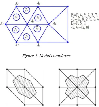
Let an arbitrary triangulation (i.e. N nodes A1,...,ANand M trianglesT1,...,TM ) of a plane region is given. Let a nodal complex Cn be a set of triangles sharing node An. Denote by n a set of triangle numbers in complex Cn; by np – a set of triangle numbers in intersection of complexes Cn and Cp (i.e. npn p); by [ ]n – a set of vertex numbers in complex Cn; by ] [m – a set of node numbers of triangular Tm. Figure 1 illustrates these denotations.
Figure 1: Nodal complexes.
Figure 2: Nodal finite elements with 7 and 9 nodes.
The idea of stabilized nodal averaging can be demonstrated by the simplest example – plane strain problem with small elastic strain. Let u=(u1,u2 ) be a FEM-approximation of the displacement field. Define average defor-mation εn at node An and average area Sn as
n
i i i
n wε
ε and Sn Sn/3 (1)
where εi – deformation on triangle Ti (εi const because Ti is a linear finite element); wi si/Sn – weight coefficient; si – area of Ti; Sn– area of Cn. Write the discretized variational equation taking into account (1):
u f ε C ε ε
C C
ε
m m
M
m m
n n
N
n n
s
S
1
where the first sum corresponds with nodal complexes while the second one – with triangles; f is an external load;
C is the isotropic elasticity tensor and C is the stabilization tensor (on optimal choice of C see Puso and Solberg (2006)).
It is clear that the influence of the stabilization tensor drops as a finite element mesh is refined but for a coarse mesh tensor C becomes to be necessary. Formally, one can consider that the tessellation procedure follows the meshing one and new finite elements appear while each of them is a one-third of a nodal complex – see Figure 2 where one-thirds of triangles (each of triangles is dissected into three parts of equal area) form a new (nodal aver-aged) finite element. Note that all the nodes except for the central one are located outside the new finite element.
As for the axisymmetric event, a volume formula for a ring of triangular profile is not so trivial as for triangular or tetrahedron. This results in too cumbersome expressions for both nodal force and stiffness matrix. In the present work, an approximate formula of volume for such a ring is exploited in order to simplify a program code and to accelerate calculations. Turn to the axisymmetric formulation itself. In cylindrical coordinates y1= r, y2= h,
=
y3 , the Cauchy stress tensor and the small strain one take the form (here, the small displacement field )
, (ur uh
u at any time interval [ ,t t t] is meant)
0 0 0 0 h rh rh r σ , r u u u u u u u r h h r h h r r h h r r r / 2 0 0 0 2 0 2 2 1 , , , , , , ε (3)
It is necessary to rewrite the variational principle (2) taking into account large irreversible (plastic) strain and the cpecific form (3) of tensors σ and ε (the Euler approach is adopted throughout the work i.e. all tensor fields refer to the current configuration rather than the initial one):
u f ε σ ε
σ
m
M
m m m
n N
n n n
v V
1 1
(4)
where
n
i i i
n wσ
σ – average stress at nodeAn;
m
σ – stabilizing stress on triangleTm;
n
i i i
n wε
ε – average strain at node An;
n i i v V
w / – weight coefficient of Ti in nodal complex Cn;
3 /
n
n V
V – averaged nodal volume;
n m m n vV – volume of nodal complex Cn;
m m
m r s
v 2 – approximate volume for a ring of triangular profile Tm; 3
/ ) (r1 r2 r3
rm – average radius of a ring of triangular profile Tm.
Equation (4) has to be supplemented by a constitutive equation. As far as metals and alloys refer to near rigid-plastic materials, it is convenient to write that equation by means of any corotational rate “r” (for example, Yau-mann’s rate “j”):
d C C σ( )
r , rσC d (5)
where d is the deformation rate tensor. Therefore, two stress tensors take part in step-by-step numerical analysis: real stress σ and stabilizing stress σ .
Introduce a FEM-approximation for the displacement field u, its gradient , and circular deformation 33:
) , (y1 y2 N
u
ui ni n ; u,ij uniNn,j(y1,y2) (1i,j2); 33ur/ru1nNn(y1,y2)/y1 (6)
where the summation over repeated indexes is implied ; the differentiation sign is separated by a comma;
) , (y1 y2
Nn – shape function corresponding to node An; (u1n,un2) – nodal displacement of An. In the sequel, a shape
function will be numerated by a pair of indexes: Nnm(y1,y2) where n corresponds to node An and m – to triangle m
T . Define an average nodal gradient as
n m i m j n m i nj w u i j
u,( ) ,( ) (1 , 2) (7)
where u,(jn)i and u,(jm)i correspond to node An and triangle Tm respectively. FEM-approximation of (7), based on approximation (6), yields
nm p n p n
n pj i p pn m m j p n m i p i p m p m j p n m i n
j w N u u w N u B i j
u (1 , 2)
] [ , [ ] [ ] , ) ( , (8)
while the summation in the last but one sum runs over the intersection of nodal complexes Cp and Cn (this intersection can be empty, consists of one or two triangles or coincides with the entire nodal complex if np); matrix B(n) is of the form
pn m m j p n m npj w N
B , (9)
Circular deformation 33 is calculated according to
1 33 [ ] n p p p n
u B
(10)where vector B~(n) is of the form
pn m m p n m np w N y y y
B~ ( 1, 2)/ 1 (11)
Due to the approximate formula for volumevm, expression (9) yields
2) , (1 2 ,
D V b i j
b s r V D b V v N w
B pjn
n m m pj pn
m m m
n m m pj pn m n m pn m m j p n m n pj (12)
where Dm2sm; mpj pn
m m
n
pj r b
b
; b(m) is the well-known in FEM matrix of coordinate differences of triangle
vertices (three nodes are numerated by 1,2,3 counter clockwise and index m is omitted):
1 2 2 1 3 1 1 3 2 3 3 2 x x y y x x y y x x y y
b . (13)
As for expression (11), taking into account the one-point integration scheme for the classical linear triangle element, function Npm(y1,y2)/y1 should be evaluated at the center of triangle Tm where this function equals to
) 3 /(
1 rm such that
n p n pn m m n pn
m n m
m n
p Vvr V s V b
B ~ 3 2 3 2 3 1 ~
(14)where
pn m m p n n
p b s
b~ ~ .
) 2 , 1 ( /
~ 1 33 1
, ]
[ [ ]
33
1
V B σ V B σ v N σ v σ N y i j
f
p
m m p
m p m m i ij m m j p m p
n n p n
n p n i ij n n pj n i
p (15)
where ij is Kronecker’s delta-symbol. Substituting (12) and (14) into (15) and taking into accountVn Vn/3,
obtain ) 2 , 1 ( 3 2 ~ 9 2
3 [ ] 1 [ ] 33 1 33
j i σ s σ b r σ b σ b f pm m p m m
i ij m m pj m p
n n p n
n p i ij n n pj i
p (16)
Point out that this expression is simpler than (15) because all volumes (both nodal and of rings of triangular profile) disappeared due to the successful choice of the approximate formula for volume vm (see the elucidations to equation (4)). Finally, a stiffness matrix is obtained by means of the nodal force variation. To this goal, find the stress tensor variation from the constitutive equation (5) with Yaumann’s rate:
σ ω ω σ d C C σ ω ω σ σ
σj ( ) ; (17)
σ ω ω σ d C σ ω ω σ σ
σj (18)
where ω(vvT)/2 is the vortex tensor. According to (17), the nodal stress variation at node An is
2) , , , (1 ) ( 2 1 ) ( ] [
u B B B B i j k l
C C σ n q n ql li n j k n ql lj n i k n qj ik n n qi kj n k q n kl ijkl n ijkl n ij
n (19)
where n denotes “no summation” over index n. Besides, matricies bn (see (12), (13)), matrix b~ (see (14) with
comments), and scalars rm,sm are also dependent variables and subjected to variation. Therefore, the total expression for the nodal force (16) variation is too cumbersome and consists of two items: symmetrical and non-symmetrical. In practice of metal forming analysis, a non-symmetrical item can be rejected without the loss of convergence. A symmetrical positively defined item of the stiffness matrix of the nodal finite element is obtained by the first item in the right hand of (19) and is of the form (p and q are node numbers of complexCn)
) 2 , , , 1 ( ) ( 3 2 )
( b C C b i j k l
V
K pjn nijkl nijkl qln n
pi qk
n (20)
while if
i
1
ork
1
then some special items should be added to the stiffness matrix respectively:n p kl n kl n n ql n p qk
n b C C b
V
K ( )~
9
2 2 33 33
1 )
(
or pjn nij nij qn
n pi q
n b C C b
V
K ( )~
9
2 2 33 33
1 )
(
(1i,j,k,l2) (21)
and if
i k
1
then one more item should be added:n q n n n p n p q
n b C C b
V
K ~ ( )~
27
4 2 3333 3333 1
1 )
(
. (22)
When assembling the global stiffness matrix, the stabilizing matrices are also taking into account (they are calculated according to classical expressions in Zienkiewicz (1971) and constitutive equation (18)). This completes the nodal averaged axisymmetric finite element formulation.
3 NUMERICAL EXAMPLES
)) (
( ij kl ik jl il jk ijkl p
C (23)
where p is a small penalty parameter (p=0.05 is recommended) and Lame’s constants and are defined in the following way. For elastic material with Lame’s constants and:
and min(,25). (24)
For plastic materials, a shear modulus based on the plastic tangent modulus ET is used: 2
/ T E
and min(,25). (25)
A contact problem statement conforms to Morrev (2007, 2009, and 2011). Only the symmetrical positively defined items (20), (21), (22) of the finite element matrix are evaluated.
3.1 Cylindrical billet upsetting
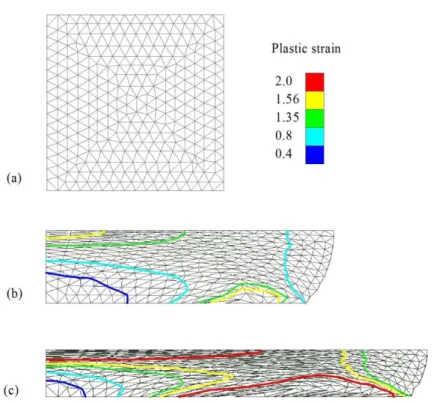
Figure 3: Upsetting of cylindrical billet. Effective plastic strain is shown for three different thicknesses: (a) 2 in; (b) 0.82 in; and (c) 0.5 in.
In this example, which is adopted in Puso and Solberg (2006), performance on a large deformation, confined plasticity problem is evaluated. The undeformed steel (E =2.987×10⁴ ksi, ν=0.3) billet is 2 in in height and diame-ter and quardiame-ter symmetry triangular mesh model is used for simulation as seen in Figure 3. The billet is squashed by two parallel rigid plates to thickness 0.5 in. A contact surface of type “stone wall” (i.e. with infinite frictional coefficient) is used to vertically constrain the outer boundary as it expands (bulges) horizontally. The material is elastoplastic with the power law hardening of the form
0113 . 0 )
112 / 41 ( ksi, )
( 112 )
( 0 0.227 0 1/0.227
y p p . (26)
In this example, the tangent modulus ET , which is used in stabilizing tensor C , was the tangent of the power law equation evaluated at εp=0:
ksi 813 )
0113 . 0 )( 227 . 0 ( 112 ) 0 ( d
d 0.773
py
T
The only difference from the original work by Puso and Solberg (2006) in the problem statement is the optimal penalty parameter value p=0.01 instead of p=0.05. That is, the axisymmetric finite element and the tetrahedral one are not identical in spite of identical meshes and common theoretical framework! The results are presented in Fig-ure 3 where the smoothing procedFig-ure (see Section 1) was applied twice to both the isoline patterns. It is difficult to compare these isolines with the results by Puso and Solberg (2006) because in that work color pictures were used to visualize the tensor fields. Nevertheless, the qualitative similarity is evident.
3.2 Deep rolling of a steel rod
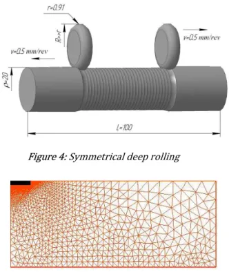
A surface hardening process of a steel rod by means of deep rolling (DR) is studied. DR is an extremely complex process (see for example Radchenko et al. (2015) and Gryadunov et al. (2015)) because of high gradient values of tensor fields and due to the induced non-uniformity of a material. As a rule, such problems are solved in a three-dimensional statement (despite a workpiece looks like an axisymmetric body) when a small representative part of a detail is considered together with some reasonable boundary conditions. In contrast to this approach, the pro-posed axisymmetric finite element permits to consider the entire detail in some events. The point is that a shape of a contact zone depends on ratio R/r where R is longitudinal roller’s radius and r is transversal one. If Rrthen the contact zone is, roughly speaking, round and the material flows in all directions from under the roller. But, if Rr then the contact surface is of the form of a very oblong oval hence the material flow is negligible in the direction of rolling and predominates in the direction of the workpiece axis, i.e. the flow character is the same as in axial sym-metric models. Consequently, a three dimensional model can be reduced to axial symsym-metric one if radius R is suffi-ciently large. The computation time diminishes drastically in such case. Turn to an appropriate example. A steel rod of radius 20 mm and of length
l
100
mm is rolled by two rollers of transverse radius r0.908mm and of longitu-dinal oneRr while the rollers move in opposite directions (Figure 4). Note once again that if Rr then the problem cannot be considered as an axial symmetric one. Rolling depth h0.15 mm; rolling step d=0.5 mm; num-ber of passes is equal to 1. Material is steel AISI 4340; hardening law is 0bn (i.e., slightly different from (26), (27)) where 0792MPa; b510MPa; n0.26; Young’s modulus E 210GPa; Poisson’s ratio 0.324.Figure 4: Symmetrical deep rolling
Figure 5: Finite element mesh
2 /
T E
. The penalty parameter value p=0.05 instead of p=0.01 in the previous example. The residual stress component along the rod axis is to be found.
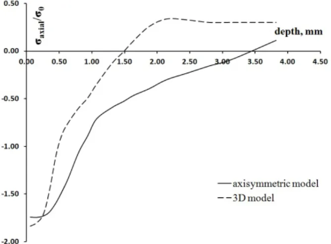
A like problem was investigated in Majzoobi et al. (2010) with the only difference: longitudinal radius was equal to R2.5 mm. The results of both the works are compared in Figure 6. The peak values are almost equal. The difference between the two plots is explained by different values of radius R. It is obvious that if Rr then the contact zone is of the form of a very oblong oval and is much larger than in case R2.5 mm. Correspondingly, the penetration depth of plastic deformation is larger too whenRr. It should be pointed out that the three-dimensional model in Majzoobi et al. (2010) was calculated up to depth 3 mm only and in the present work an extrapolation of those results up to depth 4 mm is used. The developed finite element permits to evaluate the re-sidual stress without any restriction in depth and a proper result is presented in Figure 7.
Figure 6: Axial residual stress up to deph 4mm
Figure 7: Axial residual stress along the entire deph
4 CONCLUSIONS
detail under working rather than its small three-dimensional part with considerable reduction in computation time and input data preparing.
ACKNOWLEGEMENTS
Special thanks to E. Yu. Beregovaya for her assistance in program code debugging and for developing of pre- and post-processors.
The work was carried out within the bounds of the Russian Federation government target 1.5265.2017/БЧ Nº1.5265.2017/8.9.
References
Areias, P. M., Antonio, C. A., Fernandes, A. A. (2003). Analysis of 3d problems using a new enhanced strain hexahe-dral element. International Journal for Numerical Methods in Engineering. 58: 1637–1682.
Beissel, S., Belytschko, T. (1996). Nodal integration of the element-free Galerkin method. Computer Methods in Ap-plied Mechanics and Engineering. 139: 49–74.
Bonet, J., Marriot, M., Hassan, O. (2001). An averaged nodal deformation gradient linear tetrahedral element for large strain explicit dynamic applications. Communications in Numerical Methods in Engineering 17: 551–561 Brenner, S. C., Scott, L. R. (2008). The Mathematical Theory of Finite Element Methods (Third Edition). Springer. New York.
Broccardo M., Micheloni M., Krysl P. (2009) Assumed-deformation gradient finite elements with nodal integration for nearly incompressible large deformation analysis. International Journal for Numerical Methods in Engineering. 78:1113-1134.
Chen, J. S., Wu, C. T., Yoon, S., You, Y. (2001). A stabilized conforming nodal integration for Galerkin mesh-free meth-ods. International Journal for Numerical Methods in Engineering. 50: 435–466.
Cueto, E., Chinesta, F. (2015). Meshless methods for the simulation of material forming. International Journal of Material Forming. 8: 25–43.
Dohrmann, C. R., Heinstein, M. W., Jung, J., Key, S. W., Witkowski, W. R. (2000). Node-based uniform strain elements for three-node triangular and four-node tetrahedral meshes. International Journal for Numerical Methods in Engi-neering 47: 1549–1568.
Gee, M.W., Dohrmann, C.R., Key, S.W., Wall, W.A., (2009). A uniform nodal strain tetrahedron with isochoric stabili-zation, International Journal for Numerical Methods in Engineering. 78: 429–443.
Gil, A. J., Lee, C. H., Bonet, J., Aguirre, M. (2014). A stabilised Petrov–Galerkin formulation for linear tetrahedral elements in compressible, nearly incompressible and truly incompressible fast dynamics. Computer Methods in Applied Mechanics and Engineering. 276: 659–690.
Gryadunov, I. M., Radchenko, S. Yu., Dorokhov, D. O., Morrev, P. G. (2015) Deep Hardening of Inner CylindricalSur-face by Periodic Deep Rolling - Burnishing Process. Modern Applied Science 9: 251–258.
Lee, C. H., Gil, A. J., Bonet, J. (2014). Development of a stabilised Petrov–Galerkin formulation for conservation laws in Lagrangian fast solid dynamics. Computer Methods in Applied Mechanics and Engineering. 268: 40–64.
Majzoobi, G.H., Teimoorial Motlagh S., Amiri, A. (2010). Numerical simulation of residual stress induced by roll-peening Transactions of The Indian Institute of Metals 63: 499–504.
Morrev, P. G. (2007). A Version of Finite Element Method for Frictional Contact Problems. Mechanics of Solids 4: 640–651.
Morrev, P. G. (2009). A rate variational principle of quasistatic equilibrium for absolutely rigid body in contact problems. Fundamental and applied problems of technique and technology 6: 30–32. [in Russian]
Morrev, P. G. (2011) A variational statement of quasistatic “rigid-deformable” contact problems at large strain in-volving generalized forces and friction. Acta Mechanica 222: 115–130.
Puso, M. A. (2000). A highly efficient enhanced assumed strain physically stabilized hexahedral element. Interna-tional Journal for Numerical Methods in Engineering. 49: 1029–1064.
Puso, M. A., Solberg, J. (2006). A formulation and analysis of a stabilized nodally integrated tetrahedral. Interna-tional Journal for Numerical Methods in Engineering 67: 841–867.
Puso, M. A., Chen, J. S., Zywicz, E., Elmer, W. (2008). Meshfree and finite element nodal integration methods. Inter-national Journal for Numerical Methods in Engineering 74: 416–446.
Quak, W., van den Boogaard, A. H., Gonsales, D., Cueto, E. (2011). A comparative study on the performance of mesh-less approximations and their integration. Computational Mechanics. 48: 121–137.
Radchenko, S.Yu., Dorokhov, D.O., Gryadunov, I. M. (2015). The volumetric surface hardening of hollow axisymmet-ric parts by roll stamping method. Journal of Chemical Technology and Metallurgy 50: 104–112.
Reese, S. (2002). On the equivalence of mixed element formulations and the concept of reduced integration in large deformation problems. International Journal of Nonlinear Sciences and Numerical Simulation 3: 1–33.
Reese, S. (2005). On a physically stabilized one point finite element formulation for three-dimensional finite elas-toplasticity. Computer Methods in Applied Mechanics and Engineering 194: 4685–4715.
Simo, J. C, Armero, F. (1992). Geometrically nonlinear enhanced strain mixed methods and the method of incom-patible modes. International Journal for Numerical Methods in Engineering. 33: 1413–1449.
Simo, J. C, Armero, F., Taylor, R. L. (1993). Improved versions of assumed enhanced strain tri-linear elements for 3d-finite deformation problems. Computer Methods in Applied Mechanics and Engineering. 110: 359–386. Simo, J. C, Taylor, R. L., Pister, K. S. (1985). Variational and projection methods for the volume constraint in finite deformation elasto-plasticity. Computer Methods in Applied Mechanics and Engineering 51: 177–208.
Sussman, T., Bathe, K. J. (1987). A finite-element formulation for nonlinear incompressible elastic and inelastic anal-ysis. Computers and Structures 26: 357–409.