A SOLUTION FOR A PHASE CHANGE TRANSIENT HEAT TRANSFER PROBLEM USING AN ELECTRONIC SPREADSHEET

A SOLUTION FOR A PHASE CHANGE TRANSIENT HEAT TRANSFER

PROBLEM USING AN ELECTRONIC SPREADSHEET

USO DE PLANILHA ELETRÔNICA NA SOLUÇÃO DE UM PROBLEMA DE TRANSFERÊNCIA DE CALOR TRANSIENTE COM MUDANÇA DE FASE

Luís Edson Saraiva, Cássio Alberton e Margarete Maria Trevisan

Faculdade de Engenharia e Arquitetura, Universidade de Passo Fundo, BR 285, Km 171, 99001-970 - Passo Fundo/RS. E-mail: saraiva@upf.br

ABSTRACT

Numerical solutions for heat transfer problems are usually obtained using an algorithm implemented in a sequential programming language. Despite a powerful set of tools that can be useful in many heat transfer problems, electronic spreadsheets have not been used in these sorts of problems, except for less complex issues. That is partially due to the dificulty in simulate loop iterations in electronic spreadsheets. In the present work a relatively complex phase change transient heat transfer problem is solved by coupling the spreadsheet iteration facility with the time increase required by the problem’s physics. Besides, the energy conservation equation is written based on an enthalpy formulation and the finite volume method is used for the discretization of the corresponding differential equation.

Keywords: Heat Transfer, Electonic Spreadsheet, Phase Change

RESUMO

Soluções numéricas para problemas de transferência de calor são normalmente obtidas mediante a implementação de um algoritmo seqüencial em uma linguagem computacional de alto nível. Apesar de possuírem um poderoso conjunto de ferramentas, as quais podem ser úteis em muitos tipos de problemas de transferência de calor, planilhas eletrônicas não têm sido muito utilizadas em tais problemas, exceto em algumas situações muito simples. Isto se deve, parcialmente, à dificuldade de simular iterações em laço em planilhas. No presente trabalho um problema de transferência de calor transiente com mudança de fase, de relativa complexidade, é resolvido por meio do acoplamento da funcionalidade iteração, disponível em planilhas, com o incremento no tempo requerido pela física do problema. Além disso, a equação da conservação da energia é escrita baseada em uma formulação entálpica e o método dos volumes finitos é usado para a discretização da equação diferencial correspondente.

Palavras-chave: Trasferência de calor, Planilha Eletrônica, Mudança de fase

1. INTRODUCTION

Electronic spreadsheets are generally used as an important tool in the engineers’ calculations. Also, due to their spread availability and a whole set of functionalities, spreadsheets are extensively used as an education and training tool in Engineering undergraduate courses. However, spreadsheets have inherent limitations. For instance, loops, so commonly implemented in programming languages, are hard to mimic in spreadsheets. For these reasons, there are lots of articles concerning the use of spreadsheets in scientific education, mainly about either new uses in problem solutions or about overcoming such limitations. See, for example, Tabor (2004), Mokheimer and Antar (2000), Kang

(1999), Tai (1999), Schumack (1997) and Gretton et al. (1997). The present work shows the use of an Excel™ spreadsheet in the solution of a somewhat complex heat transfer problem with a simple approach to deal with loops. As an example, a transient two-dimensional heat transfer problem with phase change is formulated and solved.

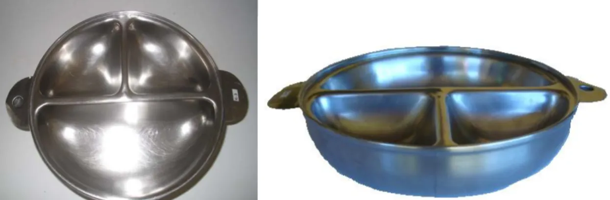
Phase change materials (PCM) are ordinarily used for energy storage, employing their latent heat, being particularly useful in applications that require heat transfer at (nearly) constant temperature. The example shown in this work aimed at the use of a PCM, inside a hollow metallic dish which can be used to deliver meals to patients at a hospital (see Fig. 1). Currently, hot water is used to keep food warmed during the time required between the dish supply and its delivery.

Figure 1 – Hollow metallic dish used for meal delivery at hospitals.

2. MATHEMATICAL FORMULATION

Cylindrical geometry is used for the heat transfer problem formulation. The equation for the transient, two-dimensional heat transfer problem considered is:

t T c z T r T r k r T k p _           _ 2 2 2 2 . (1)

A phase change process at constant pressure implies also constant temperature. So, temperature should be replaced, in Eq. (1), by an appropriate new dependent variable that could vary including the phase change period. Enthalpy usually substitutes temperature in such processes. The enthalpy transforming model employed in the present work follows the work of Cao and Faghri (1989). Enthalpy and temperature are related by:

hc_pT. (2)

In this work, enthalpy will be considered zero at the phase change temperature in the solid phase. Hence, at temperatures below the melting temperature (T < Tm), at the solid phase, enthalpy will be negative (h < 0). Throughout the phase change process (T = Tm), enthalpy varies from zero to L (latent heat). In the liquid phase (T > Tm), enthalpy assumes positive values above the latent heat value (h > L).

It is also convenient, in the current formulation, to use the so-called Kirchhoff’s temperature, defined as:





_

Therefore, Eq. (1) can be restated as: t h z T r T r r T            _ 2 * 2 * 2 * 2 1 , (4)

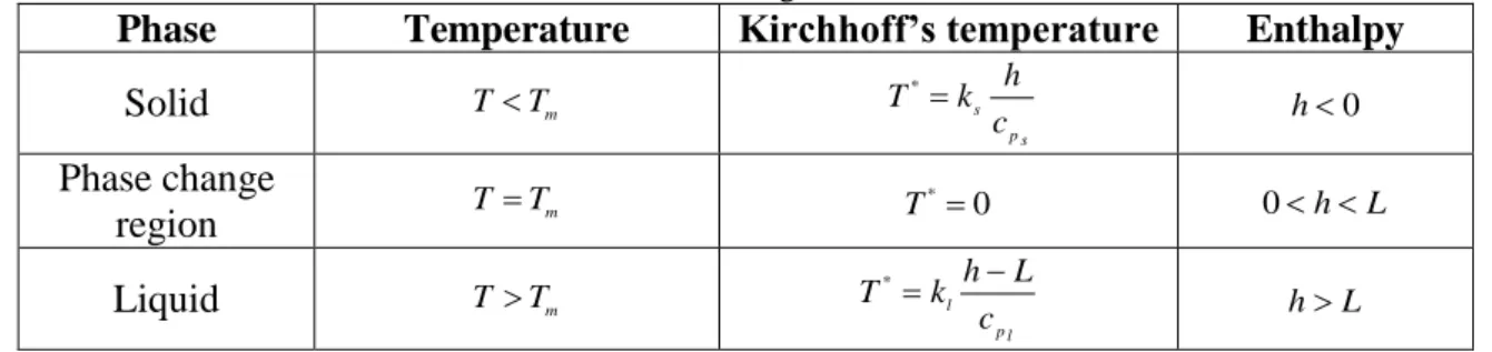
where T* and h will behave as stated at Tab.1. The subscripts l and s refer to liquid and solid phases, respectively.

Table 1 – Relationship among temperature, Kirchhoff’s temperature and enthalpy at solid, phase change and liquid regions.

Phase Temperature Kirchhoff’s temperature Enthalpy

Solid TTm s p s c h k T* 0  h Phase change region TTm 0 * T 0hL Liquid TTm l p l c L h k T*  L h

Due to numerical reasons, it will be useful to express the Kirchhoff’s temperature as a linear function of the enthalpy:

T*hS, (5) where the constants and S go after Tab. 2.

Table 2 – Constants from the linearization of the Kirchhoff’s temperature at the solid, phase change and liquid regions.

Phase Kirchhoff’s temperature constants Enthalpy

Solid s p s c k   _{S0 h0} Phase change region 0 S0 0hL Liquid l p l c k   l p l c Lk S _hL

Replacing Eq. (5) into Eq. (4), the following equation is obtained:

t h z S z h r S r r h r r S r h                                          _ 2 2 2 2 2 2 2 2 ) ( 1 ) ( 1 ) ( _{. (6)}

Equation (4) has been transformed into Eq. (6), a non-linear equation with a single dependent variable h. There is no closed form solution for Eq. (6). Hence, a numerical solution should be sought. In the present work the Finite Volume Method (FVM), (Patankar, 1980; Maliska, 2004) has been chosen.

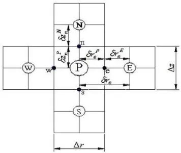
Using the FVM, the heat transfer equation is integrated for each single finite volume, being the thermodynamics properties values considered constant inside the volume. Furthermore, each finite volume is constructed around a nodal point, which concentrates the properties values. Schematic

representations of a finite control volume constructed around a nodal point “P”, and its neighbor volumes “N” (north), “S” (south), “E” (east) and “W’ (west), are shown in Fig. 2 and Fig. 3.

Figure 2 – Schematic representation of the finite control volumes (lateral view of the hollow metallic dish).

Figure 3 - Schematic representation of the finite control volumes (superior view of the hollow metallic dish).

A control volume “P” has six neighbors. However, as there is no temperature (and enthalpy) variation for the same radius, there is also no need to define the corresponding volumes. For this reason, Fig. 3 represents a fraction of the whole domain corresponding to an angle of 1 rad. Figure 4 is a general two-dimensional representation of the conventions used further.

A general algebraic equation, to be numerically solved for the domain, can be obtained by integration of the Eq. (6) with respect to the independent variables r, z and t.

The first term:

r z t r S S r h h r S S r h h dt dz dr r r S r h w W P w W W P P e P E e P P E E t t t n s e w                  _          _              

 

The second term:

z t r S r S r r h r h r r S r S r r h r h r dt dz dr r r S r r h r e P P w W W w w P P P w W W W w e E E e P P e w E E E e P P P e t t t n s e w                    _            _              

 

The third term:

t r r z S S z h h z S S z h h dzrdrdt z S z h s S P s S S P P n P N n P P N N t t t e w n s                  _          _              

 

The fourth term:

dtrdrdz





 

After the integration of Eq. (6), shown from Eq. (7) to Eq. (10), and some rearrangement, one obtains an algebraic equation as shown by Eq. (11):

AhPBhWChEDhNEhSF0, (11) where:                                                  t z z z r r r r r r r r r t z r r A s n w e w P w e P e P          1 1 1 1 1 1 1 1 , (12) _              w W w w W r r r r r r t z r r B    1 1 1 , (13) _              e E e e E r r r r r r t z r r C    1 1 1 , (14) _            n N z z t z r r D  1 1 , (15)

            s S z z t z r r E  1 1 , (16)                                            _P w e s n w P w e P e _S r z z z z z r r r r r r t z r r F 1 1 1 1 1 1 1                                            t t P S s N n E e E e e W w W w w h t S z S z z S r r r r r r S r r r r r r          1 1 1 1 1 1 1 . (17)

Finally, the enthalpy at the internal finite control volume “P” can be obtained by the following equation: A F Eh Dh Ch Bh h W E N S P       . (18) 2.1 Boundary Conditions

Equation (11) and its coefficients defined by Eq. (12) to Eq. (17) are valid for any internal node. It is necessary, however, to establish appropriate equations for the boundary conditions.

Finite control volumes, at the external surface on the hollow metallic dish, exchange heat by convection with the surrounding environment. So, one has:

V





at a rate governed by the Newton’s law for cooling:

qAc





Combining Eq. (19) and Eq. (20), and replacing temperature for enthalpy, one has:

t c h T V A h h p t t c t t t               _    . (21)

Finite control volume can be written as:

VAcl, (22)

where l is the length of a finite control volume, perpendicular to Ac. Depending on the case, l can be replaced by r or z. Equation (21), written for a finite control volume “P” at the external surface on the hollow metallic dish, therefore, could be restated as:

_             _  p t t P t t P t P c h T l t h h   (23)

Symmetry condition at the very center of the hollow metallic dish can be easily stated as:

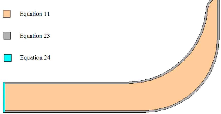
The complete set of equations for the whole domain can be visualized in Fig. 5.

Figure 5 – Equations used for different regions.

3. USING ELECTRONIC SPREADSHEET TO SIMULATE THE HEAT TRANSFER PROBLEM

The simultaneous solution of the complete set of equations was carried out using Excel™ spreadsheet. In this implementation, each finite control volume corresponds to an Excel’s cell. Excel™ has a huge number of tools and functionalities, some of them, extensively used in the present work such as conditional formatting, iteration and the function “IF”.

Iteration (Tools → Options → Calculations → Iteration (on)) was used in order to establish the enthalpy field, for the whole domain, at each time step.

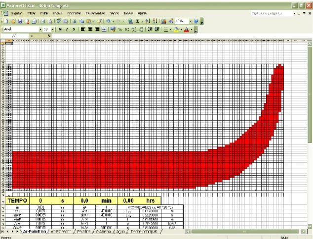
Conditional formatting was used to allow phase change processes to be visualized. Then, if a cell is “solid” it is painted in blue, if it is “liquid” it is painted in red and if the cell is “melting/solidifying” it will be painted in purple. So, throughout the iterations, the cells’ colors change.

Function “IF” was extensively used in nested statements, mostly to provide the correct value of some physical properties. For instance, if a cell were “solid”, the use of the function “IF” would allow selecting the set of values for the physical properties corresponding to the solid region, and so far. For a cell under “melting/solidification”, function “IF” would allow to calculate, automatically, an average mean for the values of the properties. For example, the average mean to the PCM’s specific mass for a cell “melting/solidifying” would be calculate as:





As one can expect from Eq. (25), if h= 0, sl=sand if h= L, sl=l.

In order to link the Excel’s iterations to time increasing, a simple but effective calculation is performed at every single iteration. The amount of energy stored into the PCM at a time t is equal to the sum of the enthalpy of each cell. In the same fashion, the total heat transfer rate can be easily obtained as the sum of the heat transfer rate released by each cell at the external surface, as stated by Eq. (20). Therefore, following and adapting Eq. (21) to the whole domain one obtains:

            _    p t t su rfa ce c t t t p a st p resen t c h T A H H t t  (26)

where tpresent and tpast are the current time and the time one step before, respectively. Also, hsurface is the PCM’s specific enthalpy on the exterior surface.

The convection heat transfer coefficient was calculated considering natural convection to the air at 20°C. It was used the following correlation to obtain the Nusselt number:





where Nu, Gr and Pr are the Nusselt, Grashof and Prandtl numbers, respectively. Nusselt number and convection heat transfer coefficient are related by:

k

Nu  (28)

where  is a characteristic dimension of the body. In the present work it was adopted the harmonic mean of the diameter and height of the dish.

4. PHASE CHANGE MATERIAL

The PCM chosen for the present application should satisfy a set of requirements. An important requirement to be met is that Tm should be between 60°C and 65°C in order to avoid the excessive proliferation of microorganisms into the food. Other important requirements for the PCM are: to own a large latent heat, to be non-toxic and not to be expensive or unavailable.

A material that meets the above requirements is the palmitic acid. The palmitic acid is a saturated fat, found in animals and plants. The main commercial source of the palmitic acid is the palm tree oil. It presents a melting temperature of 61°C, latent heat of 203.4 kJ/kg, thermal conductivity of 0.16 W/(mK), specific mass in the solid and liquid phases of 942 kg/m³ and 862 kg/m³, respectively, and specific heat in the solid and liquid phases of 2.2 kJ/(kgK) and 2.48 kJ/(kgK), respectively (Sari and Kaygusuz, 2002).

5. RESULTS

Numerical tests were performed to find appropriate space and time intervals. Results indicate the following intervals as adequate: rz0,001 m e t1s.

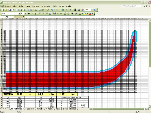
Below, a number of computer screens (Fig. 6 to Fig.10) representing the solidification process to different periods of time is shown.

Figure 6 shows an Excel™ screen representing an 1 rad slice of the metallic dish (not shown) fulfilled of PCM, before the start of the iterations. The PCM (palmitic acid) is completely molten, at 65°C, being the liquid phase represented in red. Figure 7 shows the very beginning of the solidification process, being the cells painted in purple representing PCM under solidification. Solidification process continues as time increases, as can be seen in Fig. 8 and Fig. 9. When the PCM becomes fully solid, as in Fig. 10, all the cells are painted in blue.

Figure 6 – PCM fully molten at initial time and initial temperature (65°C).

Figure 8 – Front of solidification advances towards the inner core of the PCM.

Figure 10 – PCM fully solid.

6. CONCLUSIONS

Numerical solution for a phase change transient heat transfer problem was found using an Excel™ spreadsheet. Besides, an enthalpy transforming model and the finite volume method were employed. At each time step the enthalpy field was calculated using the spreadsheet’s iteration facility. In order to simulate the loops that would be required to provide advances in time by implementations in high level programming languages, a simple link between enthalpy changes in time and the Newton’s law for cooling at the domain’s boundaries was performed.

As further research, the validation of the numerical results should be done by comparison with experimental data.

7. REFERENCES

Cao, Y., Faghri, A., 1989, “A Numerical Analysis of Stefan Problems for Generalized Multi-Dimensional Phase-Change Structures Using the Enthalpy Transforming Model”, International Journal of Heat and Mass Transfer, Vol.32, No. 7, pp. 1289-1298.

Gretton, H.W., Callender, J.T. and Challis, N.V., 1997, “Teaching Engineering Field Theory Using IT”, International Journal of Mechanical Engineering Education, Vol. 25, No. 1, pp. 1-12.

Maliska, C.R., 2004, “Transferência de Calor e Mecânica dos Fluidos Computacional”, Ed. LTC, Rio de Janeiro, Brazil, 453 p.

Mokheimer, E.M.A. and Antar, M.A., 2000, “On the Use of Spreadsheets in Heat Conduction Analysis”, International Journal of Mechanical Engineering Education, Vol. 28, No. 2, pp. 113-139. Patankar, S.V., 1980, “Numerical Heat Transfer and Fluid Flow”, Hemisphere Publishing

Corporation, U.S.A, 197 p.

Sari, A., Kaygusuz, K., 2002, “Thermal Performance of Palmitic Acid as a Phase Change Energy Storage Material”, Energy Conversion and Management, Vol. 43, pp. 863-876.

Schumack, M.R., 1997, “Teaching Heat Transfer Using Automotive-Related Case Studies with a Spreadsheet Analysis Package”, International Journal of Mechanical Engineering Education, Vol. 25, No. 3, pp. 178-196.

Tabor, G., 2004, “Teaching Computational Fluid Dynamics Using Spreadsheets”, International Journal of Mechanical Engineering Education, Vol. 32, No. 1, pp. 31-53.

Tai, K., 1999, “Integrated Design Optimization and Analysis Using a Spreadsheet Application”, International Journal of Mechanical Engineering Education, Vol. 27, No. 1, pp. 29-40.