Hybrid artificial intelligence algorithms for short-term load and price forecasting in competitive electric markets

UNIVERSIDADE DA BEIRA INTERIOR

Engenharia

Hybrid artificial intelligence algorithms for

short-term load and price forecasting in competitive

electric markets

Pedro Miguel Rocha Bento

Dissertação para obtenção do Grau de Mestre

Engenharia Eletrotécnica e de Computadores

(2º ciclo de estudos)

Orientador: Prof. Dr. Sílvio José Pinto Simões Mariano

Aos meus pais

e

avós

Agradecimentos

Em primeiro lugar gostaria de agradecer ao Prof. Doutor Sílvio Mariano, pela dedicação, acompanhamento e auxílio prestados ao longo da dissertação, num percurso e interesse iniciado ainda nas cadeiras de Sistemas de Energia Elétrica e Métodos de Apoio à decisão. Também uma palavra especial para o Mestre José Pombo por toda a sua disponibilidade e preciosa contribuição na elaboração desta dissertação.

Também não posso deixar de mencionar os meus pais por todo o apoio, essencial para a minha formação.

Um agradecimento aos Prof.s Doutores Rui Almeida e Rui Pacheco pelo auxílio prestado na compreensão de algumas matérias e nos recursos que disponibilizaram para a execução de simulações numéricas.

Por último um agradecimento a todos aqueles que, de uma forma ou de outra, contribuíram para a elaboração desta dissertação.

Resumo

O processo de liberalização e desregulação dos mercados de energia elétrica, obrigou os diversos participantes a acomodar uma série de desafios, entre os quais: a acumulação considerável de nova capacidade de geração proveniente de origem renovável (fundamentalmente energia eólica), a imprevisibilidade associada a estas novas formas de geração e novos padrões de consumo. Resultando num aumento da volatilidade associada aos preços de energia elétrica (como é exemplo o mercado ibérico).

Dado o quadro competitivo em que os agentes de mercado operam, a existência de técnicas computacionais de previsão eficientes, constituí um fator diferenciador. É com base nestas previsões que se definem estratégias de licitação e se efetua um planeamento da operação eficaz dos sistemas de geração que, em conjunto com um melhor aproveitamento da capacidade de transmissão instalada, permite maximizar os lucros, realizando ao mesmo tempo um melhor aproveitamento dos recursos energéticos.

Esta dissertação apresenta um novo método híbrido para a previsão da carga e dos preços da energia elétrica, para um horizonte temporal a 24 horas. O método baseia-se num esquema de otimização que reúne os esforços de diferentes técnicas, nomeadamente redes neuronais artificiais, diversos algoritmos de otimização e da transformada de wavelet. A validação do método foi feita em diferentes casos de estudo reais. A posterior comparação com resultados já publicados em revistas de referência, revelou um excelente desempenho do método hibrido proposto.

Palavras-chave

Algoritmos meta heurísticos, inteligência artificial, mercados elétricos, previsão da carga, previsão de preços da energia elétrica., programação evolucionária, redes neuronais artificiais, sistemas de energia elétrica, transformada de wavelet.

Resumo Alargado

Os sistemas de energia elétrica constituem “macro” entidades que agregam os mais diversos agentes, o espetro de operação destas entidades vai desde a produção, transmissão e distribuição e comercialização de energia elétrica. Particularizando, os mercados de energia elétrica, cuja função é a de explorar a eletricidade como bem económico, sofreram transformações abrangentes (como é exemplo o mercado ibérico), guiadas pelos conceitos de liberalização e desregulação, contrastando com estruturas até então, monopolistas e verticalizadas, na persecução de um melhor sistema.

Com esta mudança de paradigma, adveio um conjunto de normas regulatórias que introduziram novos desafios, entre os quais: mecanismos concorrenciais, gestão do mix de produção (acomodar nova capacidade de geração proveniente de origem renovável), imprevisibilidade associada a estas novas formas de geração e novos padrões de consumo (carga).

Neste contexto, os agentes de mercado assentam a sua tomada de decisão em função de modelos de previsão, em particular, a previsão da carga e dos preços de energia elétrica, sendo por isso um fator diferenciador. Neste quadro competitivo, há um forte interesse em técnicas computacionais de previsão que se revelem eficazes. No entanto as características inerentes às séries temporais da carga e dos preços (dada a sua volatilidade), resultam num acréscimo de complexidade, sendo por isso uma área de investigação muito ativa.

A literatura recente apresenta e valida a utilização de técnicas de inteligência artificial, como ferramentas de previsão eficazes, em concreto, métodos que combinem esforços de diferentes técnicas (métodos híbridos) revelam um desempenho superior. Como tal, é proposto foi um método híbrido, para a previsão da carga e dos preços da energia elétrica, para um horizonte temporal a 24 horas. O método baseia-se num esquema de otimização que reúne os esforços de diferentes técnicas, nomeadamente a transformada de wavelet, redes neuronais artificiais e diversos algoritmos de otimização, nomeadamente Particle Swarm Optimization e Bat Algorithm. No que diz respeito à utilização das redes neuronais artificiais (sua topologia) e na ausência de um paradigma ótimo, ou quase-ótimo, o método proposto determina uma topologia ótima, recorrendo a algoritmos de otimização.

Com o propósito de validar o método desenvolvido, o mesmo foi testado no mercado Português e no mercado regional de New England, no caso da previsão da carga, já na previsão dos preços o mesmo foi testado no mercado Espanhol e no mercado regional PJM. A consequente análise e comparação com resultados já publicados, em diferentes revistas de referência, permitiu validar o método hibrido desenvolvido.

Abstract

The liberalization and deregulation of electric markets forced the various participants to accommodate several challenges, including: a considerable accumulation of new generation capacity from renewable sources (fundamentally wind energy), the unpredictability associated with these new forms of generation and new consumption patterns, contributing to further electricity prices volatility (e.g. the Iberian market).

Given the competitive framework in which market participants operate, the existence of efficient computational forecasting techniques is a distinctive factor. Based on these forecasts a suitable bidding strategy and an effective generation systems operation planning is achieved, together with an improved installed transmission capacity exploitation, results in maximized profits, all this contributing to a better energy resources utilization.

This dissertation presents a new hybrid method for load and electricity prices forecasting, for one day ahead time horizon. The optimization scheme presented in this method, combines the efforts from different techniques, notably artificial neural networks, several optimization algorithms and wavelet transform. The method’s validation was made using different real case studies. The subsequent comparison (accuracy wise) with published results, in reference journals, validated the proposed hybrid method suitability.

Keywords

Artificial intelligence, artificial neural networks, electric energy prices forecasting, electric markets, electric power systems, evolutionary programming, load forecasting, metaheuristic algorithms, wavelet transform.

Contents

1 Introduction _______________________________________________________________ 1 1.1 Electric Energy Systems __________________________________________________ 1 1.2 Energy characteristics and challenges_______________________________________ 2 1.2.1 The rise of Electrical Energy ________________________________________ 2 1.3 Electrical Energy and Power _______________________________________________ 3 1.3.1 Electrical power demand (Load) _____________________________________ 3 1.4 The electric market _____________________________________________________ 5 1.4.1 The Iberian electricity market_______________________________________ 5 1.5 Time-series forecasting and (time horizons) _________________________________ 6 1.6 Load Forecast ___________________________________________________________ 6 1.7 Price Forecast __________________________________________________________ 8 1.8 Motivation and Goals _____________________________________________________ 9 1.9 Dissertation structure ___________________________________________________ 10 2 Wavelet Theory ___________________________________________________________ 11 2.1 Background ____________________________________________________________ 11 2.2 Continuous Wavelet Transform ___________________________________________ 15 Properties of Continuous Wavelet Transform ___________________________________ 16 2.3 Inverse Continuous Wavelet Transform _____________________________________ 16 2.4 Discrete Wavelet Transform ______________________________________________ 17 2.5 Inverse Discrete Wavelet Transform _______________________________________ 17 2.6 Multiresolution Analysis _________________________________________________ 18 2.6.1 Orthogonality ____________________________________________________ 19 2.6.2 Orthonormality __________________________________________________ 20 2.6.3 Orthogonal Wavelet Transform _____________________________________ 20 2.6.4 Inverse Orthogonal Wavelet Transform ______________________________ 20 2.6.5 Multiresolution Filters and Mallat Algorithm __________________________ 21 2.7 Base Wavelet (families) _________________________________________________ 22 2.8 Mother Wavelet Selection ________________________________________________ 23 2.8.1 Qualitative Criterions _____________________________________________ 23 2.8.2 Quantitative Measures/Criterions ___________________________________ 23 3 Neural Networks __________________________________________________________ 27 3.1 Background ____________________________________________________________ 27 3.2 Neural Network learning process (algorithms) _______________________________ 31 3.2.1 A review on the classical learning rules ______________________________ 32 3.2.2 Generalized Delta Rule (explained) _________________________________ 34 3.2.3 Other approaches ________________________________________________ 35 3.2.4 Scaled Conjugate Gradient Algorithm ________________________________ 36 3.3 Neural Network Architectures (configurations) ______________________________ 37 3.4 Activation Functions ____________________________________________________ 39

3.4.1 Commonly used activation functions ________________________________ 40 3.5 Other Considerations ___________________________________________________ 41 3.5.1 Weights initialization ____________________________________________ 41 3.5.2 Training Time ___________________________________________________ 42 3.5.3 Local minima problem ____________________________________________ 43 4 Optimization Algorithms ___________________________________________________ 45 4.1 Metaheuristic Algorithms ________________________________________________ 45 4.2 Particle Swarm Optimization ____________________________________________ 46 4.2.1 Implementation _________________________________________________ 47 4.3 Bat Algorithm _________________________________________________________ 49 4.3.1 Implementation _________________________________________________ 50 4.4 Cuckoo Search ________________________________________________________ 51 4.4.1 Implementation _________________________________________________ 52 4.5 Optimization algorithms as ANN learning methods ___________________________ 53 5 Load Forecast ____________________________________________________________ 55 5.1 Proposed Methodology __________________________________________________ 55 5.1.1 Input Selection and Features Extraction _____________________________ 56 5.1.2 Mother Wavelet Pre-Selection _____________________________________ 58 5.1.3 ANN Training ___________________________________________________ 58 5.1.4 ANN Architecture and Wavelet Analysis tuning _______________________ 59 5.1.5 Forecasting accuracy measure _____________________________________ 61 5.2 Case Study I __________________________________________________________ 61 5.2.1 Numerical Results _______________________________________________ 67 5.3 Case Study II __________________________________________________________ 68 5.3.1 Numerical Results _______________________________________________ 69 6 Price Forecast ____________________________________________________________ 73 6.1 Proposed Methodology __________________________________________________ 73 6.1.1 Forecasting accuracy measures ____________________________________ 74 6.2 Case Study I __________________________________________________________ 75 6.2.1 Numerical Results _______________________________________________ 76 6.3 Case Study II __________________________________________________________ 79 6.3.1 Numerical Results _______________________________________________ 80 7 Final Remarks ____________________________________________________________ 83 7.1 Conclusion ____________________________________________________________ 83 7.2 Future Works _________________________________________________________ 84 8 References ______________________________________________________________ 85 Annex A ______________________________________________________________________ 93

List of Figures

Figure 1.1 - World Growth Rate referred to 1980 value (evolution). ______________________ 3 Figure 1.2 – Spanish daily load curve (example). ______________________________________ 4 Figure 1.3 – Schematic illustration of the various methods applied in STLF and STPF. _______ 9 Figure 2.1 - Rectangular basis function example. ____________________________________ 12 Figure 2.2 - Frequency vs Time resolution. __________________________________________ 12 Figure 2.3 - Narrow to Wide Window effect in STFT [53]. ______________________________ 13 Figure 2.4 -Example of translation by a time constant τ and dilation by scaling factor s. ___ 14 Figure 2.5 - Wavelet transform process overview. ____________________________________ 14 Figure 2.6 - Wavelet (closed) subspaces. ___________________________________________ 19 Figure 2.7 - Example of DWT filter bank decomposition (tree). _________________________ 22 Figure 3.1 - Biological neuron structure (behavior). __________________________________ 28 Figure 3.2 - McCulloch-Pitts neuron model. _________________________________________ 28 Figure 3.3 - Perceptron network model. ____________________________________________ 29 Figure 3.4 - Adaline network model. _______________________________________________ 30 Figure 3.5 - Madaline network model. ______________________________________________ 30 Figure 3.6 -ANN key building blocks. _______________________________________________ 30 Figure 3.7 - Supervised Training scheme. ___________________________________________ 31 Figure 3.8 - Reinforcement training scheme. ________________________________________ 32 Figure 3.9 -Climbing the Mountain. ________________________________________________ 33 Figure 3.10 - Multiple Layer Neural Network. ________________________________________ 38 Figure 3.11 - Jordan (recurrent) Network. __________________________________________ 39 Figure 3.12 - Heaviside Step Function (σ=0). ________________________________________ 40 Figure 3.13 - Sigmoid function (σ=1) _______________________________________________ 41 Figure 3.14 - Bipolar Sigmoid function (σ=1). ________________________________________ 41 Figure 3.15 - Network performance illustration (Training/Validation error evolution). _____ 42 Figure 3.16 - Local minima problem. _______________________________________________ 43 Figure 4.1 - Metaheuristic algorithms taxonomy [74]. _________________________________ 46 Figure 4.2 - Particle position evolution (graphical overview). __________________________ 47 Figure 4.3 - Graphical representation of the most common PSO topologies. ______________ 48 Figure 5.1 - Proposed methodology (Overview) ______________________________________ 56 Figure 5.2 - Input selection process ________________________________________________ 57 Figure 5.3 - Load time series partial autocorrelation (PACF) ___________________________ 57 Figure 5.4 - Codification of the domain search space _________________________________ 60 Figure 5.5 - PSO results for BA initial settings tuning. _________________________________ 61 Figure 5.6 - Load [MW] from 1 September 2015 to 31 August 2016 (PT) __________________ 62 Figure 5.7 - Box-Plot for the monthly distribution of Portuguese load ___________________ 63 Figure 5.8 - Box Plot of load grouped by seasons on a Monday (PT) ______________________ 64 Figure 5.9 – Load box-plot grouped by seasons on a Tuesday (PT) _______________________ 64

Figure 5.10 - Load box-plot grouped by seasons on a Wednesday (PT) ___________________ 65 Figure 5.11 - Load box-plot grouped by seasons on a Thursday (PT)_____________________ 65 Figure 5.12 - Load box-plot grouped by seasons on a Friday (PT) _______________________ 66 Figure 5.13 - Load box-plot grouped by seasons on a Saturday (PT) _____________________ 66 Figure 5.14 - Load box-plot grouped by seasons on a Sunday (PT) ______________________ 67 Figure 5.15 - Forecasted load for the 7-day winter season (PT). _______________________ 68 Figure 5.16 - Load [MW] from 1 January 2016 to 31 December 2016 (NE) ________________ 69 Figure 5.17 - Forecasted load for the 7-day spring season (ISNE). ______________________ 70 Figure 6.1 - Proposed methodology (flowchart). _____________________________________ 74 Figure 6.2 – Electricity prices from 1 January 2002 to 31 December 2002 (SP) ____________ 75 Figure 6.3 - Winter week for the Spanish market: actual prices, solid line, together with the forecasted prices, dashed line. ___________________________________________________ 79 Figure 6.4 - Fall week for the Spanish market: actual prices, solid line, together with the forecasted prices, dashed line. ___________________________________________________ 79 Figure 6.5 - Electricity prices in the PJM market for the 2006 year. ____________________ 80 Figure 6.6 - Spring week for the PJM market: actual prices, solid line, together with the forecasted prices, dashed line. ___________________________________________________ 82 Figure 6.7 - Summer week for the PJM market: actual prices, solid line, together with the forecasted prices, dashed line. ___________________________________________________ 82

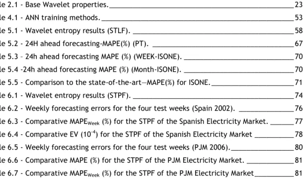
List of Tables

Table 2.1 - Base Wavelet properties. _______________________________________________ 23 Table 4.1 - ANN training methods. _________________________________________________ 53 Table 5.1 - Wavelet entropy results (STLF). _________________________________________ 58 Table 5.2 - 24H ahead forecasting-MAPE(%) (PT). ____________________________________ 67 Table 5.3 – 24h ahead forecasting MAPE (%) (WEEK-ISONE). ____________________________ 70 Table 5.4 -24h ahead forecasting MAPE (%) (Month-ISONE). ____________________________ 70 Table 5.5 - Comparison to the state-of-the-art—MAPE(%) for ISONE. _____________________ 71 Table 6.1 - Wavelet entropy results (STPF). _________________________________________ 74 Table 6.2 - Weekly forecasting errors for the four test weeks (Spain 2002). ______________ 76 Table 6.3 - Comparative MAPEWeek (%) for the STPF of the Spanish Electricity Market. ______ 77

Table 6.4 - Comparative EV (10-4_{) for the STPF of the Spanish Electricity Market __________ 78}

Table 6.5 - Weekly forecasting errors for the four test weeks (PJM 2006). ________________ 80 Table 6.6 - Comparative MAPE (%) for the STPF of the PJM Electricity Market. ____________ 81 Table 6.7 - Comparative MAPEWeek (%) for the STPF of the PJM Electricity Market __________ 81

List of Acronyms

EES Electric Energy Systems GDP Gross Domestic Product

EIA U.S Energy Information Administration MIBEL Mercado Ibérico de Energia Elétrica STLF Short-Term Load Forecast

ARMA Autoregressive Moving Average

ARIMA Autoregressive Integrated Moving Average ARCH Autoregressive Conditional Heteroscedasticity AI Artificial Intelligence

ANNs Artificial Neural Networks SVMs Support Vector Machines FIS Fuzzy Inference Systems

WT Wavelet Transform

ELM Extreme Learning Machine SARIMA Seasonal ARIMA

ANFIS Adaptive Neuro Fuzzy Inference System MAPE Mean Absolute Percentage Error STPF Short-Term Price Forecast

GARCH Generalized Autoregressive Conditional Heteroskedastic CNNs Cascaded Neural Networks

GARCH Short Time Fourier Transform CNNs Continuous Wavelet Transform STFT Short Time Fourier Transform CWT Continuous Wavelet Transform DWT Discrete Wavelet Transform MRA Multiresolution Analysis Adaline Adaptive linear neuron Madaline Multilayered Adaline MSE Mean Squared Error

MRE Mean Relative Estimation Error MAE Mean Absolute Error

SSR Sum of Squared Residuals RMSE Root Mean Square Error LMS Least Mean Squared

CG Conjugate Gradient

LM Levenberg-Marquardt SCG Scaled Conjugate Gradient

BFGS Broyden–Fletcher–Goldfarb–Shanno FFNN Feed Forward Neural Network MLP Multi-Layer Perceptron

CN Competitive Network

RN Recurrent Network

ReLU Rectified Linear Unit

PSO Particle Swarm Optimization

BA Bat Algorithm

CS Cuckoo Search

MI Mutual Information

CMI Conditional Mutual Information PAC Partial Autocorrelation

EC European Commission

REN Rede Elétrica Nacional

ISONE Independent System Operator New England REE Red Eléctrica de España

Chapter I

1 Introduction

This chapter presents a short theoretical background about Electric Energy Systems (EES) key topics and a brief state of the art review in the load and electricity prices forecasting paradigm. EES nowadays are complex systems that cover vast geographical areas and must meet high quality of service and safety standards.

Furthermore, this chapter presents the motivation behind the dissertation, main tasks and objectives are also outlined.

1.1 Electric Energy Systems

The primary goal of EES is to monetize and explore electric energy conveniently. Its development is studied by electrical engineering branches, involving aspects that include generation, transmission, distribution and consumption technologies [1].

In contemporary societies, EES are cost intensive and probably constitute the vast man made system (thousands of km of overhead lines and underground cables, as well as an endless number of elements/infrastructures [2]). They must meet a set of requisites, such as: a continuously availability, independently of the location, electricity must be generated and transmitted as it is consumed (plus loses), which means that electric systems are highly

dynamic, minimizing the production costs as well as the environmental impact, all this fulfilling a set of constrained quality norms (fault tolerance).

1.2 Energy characteristics and challenges

The energy concept is abstract but usually is defined as the capacity to produce work, energy can be classified as primary, secondary, final commercial energy or useful energy depending on the level of processing/conversion it suffered, being primary energy a not converted natural resource (e.g. fossil fuels).

Since the distant days where wood and animal muscles were the primary source of energy for mankind activities, to the present times, where energy is a crucial element that we depend unceasingly to live well, and that is why countries with higher per capita energy consumption are usually those with higher GDP (gross domestic product) per capita. In fact energy demand is closely tied with population and economic growth and based on the projected evolution of these statistical parameters, EIA (U.S Energy Information Administration) estimates that world energy consumption will grow by 48% between 2012 and 2040 [3].

This energy demand growth translates into severe constraints affecting the already scarce and increasingly costly energy resources. The expected declining in a long-term perspective for the traditional coal, gas and oil reserves and a greater attention to its underlying carbon footprint, has led to an exhaustive search and implementation of clean, renewable but also viable sources of energy.

1.2.1 The rise of Electrical Energy

Electrical energy is the result of electric potential energy or kinetic energy conversion processes. Its relatively low entropy form, which can be transmitted at long distances (electric charges flow) and converted into other forms of energy such as motion, light or heat with high energy efficiency.

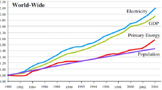
For these reasons, it’s natural when analyzing final commercial energy data, that electrical energy turned into the main energy type at the consumer end. Greatly due to its controllability, instant availability and consumer end cleanliness, doubling its demand growth in comparison with other energy types (as can be seen in Figure 1.1 [4]).

Given this consumer end preference conventional coal, oil, gas, nuclear and other resources will be gradually less used as final commercial energy source, but rather a way to generate electrical energy (process known as electricity generation).

Figure 1.1 - World Growth Rate referred to 1980 value (evolution).

Given this consumer end preference conventional coal, oil, gas, nuclear and other resources will be gradually less used as final commercial energy source, but rather a way to generate electrical energy (process known as electricity generation).

1.3 Electrical Energy and Power

As seen previously EES provide electrical energy to consumers and ensure that contracted power is available so that they can satisfy their loads (consumption). The electrical power unit (SI) is the watt (𝑊) or joule per second (𝐽/𝑠), analogously the energy is measured in joule (𝐽) or watt-second (𝑊. 𝑠). Given the real magnitude of these parameters, it’s common to use multiples like 𝐺𝑊 for power and 𝐺𝑊. ℎ for energy.

Thus we can define the relationship between energy and power as: 𝑃(𝑡) =𝑑𝑊(𝑡)

𝑑𝑡

(1.1)

𝐸(𝑡) = ∫ 𝑃(𝑡) 𝑑𝑡 (1.2)

where 𝐸(𝑡) denotes energy, 𝑃(𝑡) is power and 𝑡 is the time instant.

1.3.1 Electrical power demand (Load)

As discussed in section 1.1, EES must match in real time the power generation 𝑃𝐺 and

electric power demand D (equation 1.3).

∑ 𝑃𝐺𝑡 = 𝐷𝑡, for every time instant t

As an example Spanish power demand daily evolution (also referred as daily load curve) on February 8, 2016, is represented graphically in Figure 1.2. As would be expected from equation 1.2, the area below the curve (gray) represents the total energy.

This daily load curve varies due to a set of factors, such as the time of day, the day of the week, temperature, seasons, latitude etc. [5].

Figure 1.2 – Spanish daily load curve (example).

When analyzing a daily load curve we can highlight some points/regions of interest [5], [6], first the “peak demand” point (maximum power demand) which often occurs in early evening and typically with this increased “stress” for the generation operators it comes an high price. On the opposite way, when the minimum power demand is verified, it receives the designation of “off-peak demand” point. The period approximately between 6 and 9 AM is designated as “morning ramp”, it’s associated with the end of the night period, marking the relatively rapid transition from lower to higher power demands, and sometimes this “abrupt” transition can be stressful for EES, potentially reflecting in a greater price volatility. Another highlighted region is the red horizontal line indicating the average power for 𝑇 = 24ℎ, which is determined as follows: 𝐸(𝑡) =1 𝑇∫ 𝑃(𝑡) 𝑑𝑡 𝑇 0 (1.4)

1.4 The electric market

In the last decades, electric markets undergone trough considerable changes guided by liberalization and deregulation concepts, these changes contrast with the previous reality, where the various EES participants were “heavily” regulated by governmental hassles (public service frameworks), with highly vertical business philosophies.

This deregulation process translates into a set of policies to promote free competition markets rather than traditional monopolistic, thereby relieving to a certain extent the government control. The idea behind deregulation is to establish a more proficient market, favoring energy exchanges between markets, increasing security of supply and the main goal, reduce the costs. As a consequence of this targeted policies, available power capacity can be used more efficiently in a large region compared to a small one, whereby integrated markets enhance productivity and improve efficiency.

The first experiences occurred in Chile (1982) following a comprehensive set of economic reforms that took place during this decade, which would be later known as the "Miracle of Chile”. Subsequently in the early 90s Nordic countries restructured their electric markets and established a common Nordic market (Nord Pool Spot market), which was the world's first multinational exchange for trading electric power and today operates in Norway, Denmark, Sweden, Finland, Estonia, Latvia, Lithuania, Germany and the UK. Certain regional US markets, as well as the Australia and Iberian (Spain and Portugal) undergone trough similar restructuring processes.

1.4.1 The Iberian electricity market

In order to liberalize the electricity market, promote price stability, a better generation capacity management, increase the number of participants (consumers and producers) as well as the competition, Portuguese and Spanish governments signed an agreement in 2004 to create the Iberian electricity market (MIBEL). Entering into live mode on July 2007, becoming then only the second European regional market to be formed. MIBEL was implemented as a mixed market (pool and bilateral contracts trading) [7]. Two market operators are responsible for both dairy and intra-diary short-term market management, where the prices are determined based on the supply and demand curves.

Another particular feature of the Iberian market is that by regulatory mandate it favored a paradigm change and investments on new generation technologies (renewable energies). As such the Portuguese scenario of high energetic dependence in 2007, especially from primary energy sources (with a fossil origin), reaching values close to 83%, contrasts 9 years later (2016) with a generation of 64% of the consumed electricity by renewable sources, with a special emphasis on wind energy.

This paradigm change added significant generation capacity but also an intrinsic uncertainty arising from the nature of the renewable energies. For this reason, market participants focus is divided both on the consumption (load) and generation predictability.

1.5 Time-series forecasting and (time horizons)

A time series is a sequence of equally spaced observations in time (sequence of discrete-time observations. Considering a time-series [𝑥𝑡−𝑛, … , 𝑥𝑡−2, 𝑥𝑡−1, 𝑥𝑡], the forecasting

(or prediction) task consists in determining the upcoming (unknown) time-series values ([𝑥𝑡−𝑛+1, … , 𝑥𝑡−2+1, 𝑥𝑡−1+1, 𝑥𝑡+1]), using and modeling the existing time-series. Examples of

time-series are financial data (indices, rates etc.), weather data (temperature, wind speed, etc.), as are the load and electricity prices studied in this work.

When we speak about forecasting practices and how they are developed, one important factor is the considered temporal horizon. Consensually, forecast time horizons (for load and electricity prices) are divided into 3 large groups [8][9], to which can be added another for very short-term forecasts [10]:

 Very short-term: From scarce seconds to half an hour (one hour) prediction.  Short-term: Typically, from one hour to one week.

 Medium-term: From one week to one year.  Long-term: Longer than a year.

1.6 Load Forecast

As we saw the energy sector has evolved in the last years towards a wider, horizontal and more complex architecture, largely due to deregulation and search for efficient policies [11], [8], followed by emerging consumption patterns (with an overall growth tendency), a more deregulated supply, where the role of producer and consumer can intersect, etc. All of this has added non-linearity to the load profile [11], leading to poorly conditioned load curves, i.e. with fewer “smooth” regions, and making load forecasting more difficult, e.g. leading to worse correlations with some common exogenous variables, such as weather variables [12], which are frequently used as inputs in state-of-the-art methods [12], [13].

Short-term load forecast (STLF) is the prediction of electric load evolution, within a time horizon, with lead times extending from one hour to one week (168h) as stated in the previous section.

In such a competitive environment, STLF greatly influences decision-making on issues such as: generation scheduling (dispatch), price forecasting, need for maintenance and system liability assessment [12], [14], [15]. For these reasons researchers efforts typically focus in one day (24h) ahead load forecast. Therefore, the challenge and importance of having accurate forecast methods is even more important than before [12]. The existing literature presents a comprehensive spectrum of methodologies for STLF. To simplify they can be grouped into three different categories.

The first presents the statistical methods (time series based) and, as for other commodities, was the first conventional set of methods for STLF. This includes

autoregressive moving average (ARMA) and autoregressive integrated moving average (ARIMA); the Holt-Winters exponential smoothing; and methods based on stochastic approaches, like autoregressive conditional heteroscedasticity (ARCH) [16]–[18].

Other common method is the persistence model also known as “Naïve Predictor”, this assumes that load value in the instant 𝑡 + ∆𝑡 is the same that took place in the instant 𝑡. This is a very accurate method in very short-term horizons and loses performance when we increase the horizon (∆𝑡).

However these methods are best suited to deal with “smoother” time series, as they are not fully able to cope with the complex non-linear characteristics evidenced in the load time series [19].

To face this complex non-linearity the focus has changed to artificial intelligence (AI) methods [15], given their ability to learn nonlinear relationships between the load and exogenous variables. In this field, countless approaches have been proposed, such as: artificial neural networks (ANNs) [11], [14], [20]–[22]; random forest [19], [23]; support vector machines (SVMs) [24], [25]; fuzzy inference (expert) systems (FIS) [26], [27]; and data mining techniques [28], [29].

Despite the virtues of these AI methods, their complexity makes it hard to find the optimal parameter settings (e.g. decide ANN architecture). In addition to handicaps of each individual method, this has led us to the last category, hybrid methods. These methods take advantage of the best features of single methods. By combining them, it’s possible to explore the powerful features of each one, resulting in new topologies.

A hybrid approach is presented in [30] where an ARIMA model – used to forecast the linear load segments – is combined with SVMs – used in the forecast of the non-linear sensitive load segments.

Signal processing techniques applied to the load time series, especially wavelet transform (WT), have also been extensively employed [12], [31], [32]. The results show that wavelet analysis can extract redundant information (e.g. high frequency changes) from the load time series, resulting in a filtering effect that improves forecast accuracy [15], [33]. The concept of extreme learning machine (ELM), linked with hybrid neural networks, has also aroused the interest of researchers [13], [34]. Alternatively, in [12], [35], authors proposed hybrid structures merging ANNs, WT and optimization algorithms.

Three different methodologies were compared in [36] for very short and short-term horizons. The results show that ANNs outperforms SARIMA models and the hybrid topology ANFIS, in terms of mean absolute percentage error (MAPE (%)).

To summarize, recent literature shows that hybrid methods that combine metaheuristics algorithms, AI methods and data processing techniques are among the most accurate, although they can be computationally intensive. An overall performance comparison of these methods reveals that the MAPE for a 24h time horizon is within a 1% to 3% interval [19].

1.7 Price Forecast

As a widely spread traded commodity electricity in the form of energy blocks is sold and bought by producers and consumers who submit their bids in a pool based market, these are analyzed by the market operator which then determines the clearing price (the energy price typically on an hourly basis). But unlike other commodities electricity cannot be queued and stored economically with the exception of pumped-storage hydro plants in certain conditions [37].

Therefore, the power industry operates in a very competitive framework, largely due to deregulation and the search for competition policies with the clear intent to reduce marginal costs (and consequently obtain lower consumer electricity prices at the end of the chain). This deregulated environment brings a degree of uncertainty to electricity prices (price volatility), with profit maximization being the major concern when addressing scheduling of energy generation [37].

As such forecast accuracy is a major subject for producers and consumers. Reliable price forecasting techniques are used by the market players to derive their pool bidding strategies and to optimally schedule energy resources [37], and for this reason can be a key factor between competitors, allowing producers to maximize their profits and consumers to maximize their utilities [33]. Due to this interest forecasting electricity demand and prices has emerged as one of the major research fields in electrical engineering [38].

A set of details from the price time-series makes the task of forecasting prices far from being trivial, these include high frequency, non-constant mean and variance, multiple seasonality, calendar effect, high level of volatility and high percentage of unusual price movements [38]. Another set of details affecting forecasting accuracy is the uncertainty related with fuel prices, future additions of generation and transmission capacity, regulatory structure and rules, future demand growth, plant operations and climate changes [39]. Presently, some markets with strong penetration of renewable energy sources, particularly wind power (as the Iberian market), have special regulatory regimes (feed-in-tariff scheme) imposing new challenges that need to be accommodated, mainly due to the fluctuating feed-in of wfeed-ind power. For example, a day with prices close to zero can be followed by a day of maximum prices, which together with transmission congestion, contributes to price volatility.

A variety of methods have been developed for electricity price forecasting and most of them are also used load forecasting [38], the majority of these, as this work does, focus in lead times ranging from one hour to a week ahead forecasting, this time horizon constitutes the short-term price forecast (STPF) category.

Most methods are based in time series models, meaning that the scope is on the price time series past behavior, with addition it can be complemented with some exogenous variables. The first major approach are Parsimonious stochastic methods, for example ARIMA [40] and generalized autoregressive conditional heteroskedastic (GARCH) [41], [42] models are proposed, other time series models based on regression are presented in [43], [44]. A

Wavelet Transform is a commonly used feature to better deal with the non-constant mean and variance and the significant number of outliers is the wavelet transform. The transformed time-series presents a better behavior (more stable variance and less outliers) than the original price series thus resulting in a better performance [33]. For exemple in [33], [45] the authors combine WT with the classical ARIMA and GARCH models.

Given the limitations presented by the first set of methods, authors focused their efforts on AI methods, thus constituting the second major group of methods, this are better suited to deal with hard non-linear relationships highlighted in the price time series, thus being computationally more efficient [37]. A large portion of this AI methods are centered in ANNs , therefore authors in [37], [46], [47] used feed forward, radial basis and Elman networks in classical approaches, in [48] authors propose an improved training process for the ANN.

In order to conjugate synergies from different features the current approaches focus on hybrid methods, an example is the use of WT and a fused version of neural networks and fuzzy logic [49], in [50] the authors used cascaded neural networks (CNNs) combined with the chemical reaction optimization algorithm, to properly train the CNN, other hybrid approach was followed in [51] where the fuzzy ARTMAP, wavelet transform and firefly algorithm were used to perform the STPF.

1.8 Motivation and Goals

The existing complexity both in load and price time series makes the forecasting task far from trivial, due to a set of characteristics such as multiple seasonality, not constant mean and variance, high volatility (significant number of spikes).

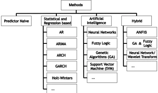
As we saw in the two previous sections, a diverse group of methods is applied both in load and price forecasting, and in a generic form, they can be grouped as illustrated in Figure 1.3.

Being a very active research area dealing with sensitive issues, and given the “rich” state of the art proposed so far, the task of exploring this diverse methods and techniques, as well in a subsequent stage, the pursuit for a contribution with a new approach, able to minimize the error compared to other reported methodologies, constitutes the major motivation behind this work. Thus the search for a STLF and STPF approach will guide this dissertation.

This new approach will fit in the hybrid methods classification (Figure 1.3), given the benefits revealed by literature review. From all the methods those who stand out and will be used are: ANN to perform the forecast, WT in a preemptive processing stage to better deal with the data series characteristics.

1.9 Dissertation structure

In this chapter a background review regarding key concepts, as well as the motivation and goals for this work dissertation were presented, the following chapters are organized in the following manner:

i. Chapter I presents a background review regarding key concepts, as well as the motivation and goals for this work

ii. Chapter II serves as a theoretical revision of the wavelet associated concepts

iii. Chapter III presents an extensive theoretical formulation of concepts associated with neural networks.

iv. Chapter IV introduces the optimization algorithms theme and the background theory behind the chosen algorithms employed in this work.

v. Chapter V and VI reveal the proposed methodology, the case studies where it was employed (STLF and STPF) and a general discussion about the achieved results. vi. Chapter VII presents the main conclusions of this dissertation.

Chapter II

2 Wavelet Theory

Numerous works related with data series analysis and particularly the ones focused in forecasting models have implemented successfully wavelet analysis, as an effective form of signal representation. So this chapter presents a comprehensive explanation of the underlying wavelet theory, from its origins, its advantages, the way it’s analytically implemented and other involving details.

2.1 Background

In 1909 with is theory of orthogonal systems, Alfred Haar was the first to conceive the idea behind what we call a “wavelet”. This groundbreaking work resulted in the discovery of a set of rectangular basis functions (what constitutes the Haar wavelet family), which are the simplest family of wavelets (Figure 2.1).

Figure 2.1 - Rectangular basis function example.

The first evident advantage is that Haar basis functions are scalable for different intervals, in contrast with Fourier basis functions which operate in the interval [-∞,+∞]. The next major contributes arrived in 70’s by the hands of Jean Morlet which successfully implemented a technique of scaling and shifting in an analysis window of a function. Morlet called the resulting waveform(s) from the analysis “wavelet(s)”. Later in 1984 Morlet partner up with Grossman to prove that a signal could be transformed to a wavelet form and then reverse the process in a procedure without information loss.

So we can define a wavelet as a small and finite wave with an irregular oscillating pattern, with finite energy. So a wavelet transform is basically a process of repeated variations of scale, translations and convolution between 2 signals, allowing the extraction of the so called wavelet coefficients.

The small scales are used to properly depict the higher frequencies and larger scales correspond to low frequency components, Figure 2.2.

Figure 2.2 - Frequency vs Time resolution.

Characteristics viewed so far reveal some distinctive traits that arise with the use of wavelets, for example, unlike short time Fourier transform (STFT), which consists in performing multiple Fourier transforms over smaller windows translated in time, where the window size is important because if the window is to narrow it results in poorer frequency resolution. Conversely a longer time window improves frequency resolution while resulting in poorer time resolution because the Fourier transform loses all time resolution over the duration of the window [52], this effect is illustrated in Figure 2.3.

Figure 2.3 - Narrow to Wide Window effect in STFT [53].

Wavelet Transform enables variable-sized windows, allowing the use of long time intervals for more precise low-frequency information, and shorter windows for high-frequency information [52], thus better for revealing hidden features in the signal, such as trends, noise detection, discontinuities in higher derivatives and self-similarity [12]. Furthermore, wavelet analysis can often compress or de-noise a signal without appreciable degradation, i.e. it has a filtering effect [12]

Figure 2.4 -Example of translation by a time constant τ and dilation by scaling factor s.

So WT decomposes the signal into a time-scale/frequency domain in a bi-dimensional analysis (time and Fourier space). As illustrated in Figure 2.4, the WT process consists in shifting a base wavelet along the signal (translation in time domain) and scale it (dilation or contraction) therefore changing the scale (which is inversely proportional to the frequency) and then, find resemblances interpreted in the form of coefficients. An overview of the complete process is illustrated in Figure 2.5, where we can see the operations both in the time and frequency domains.

Figure 2.5 - Wavelet transform process overview.

Another important step was the introduction of multiresolution analysis presented in the 10 year period between 1989 and 1999 by Mallat and Meyer, which allowed investigators

This theory led to innumerable research projects and applications, which emerged based on WT. From signal analysis, video coding [54] to image processing [55], and since is very good to extract key features from a signal it is used as an aiding mechanism in forecasting methods [34][56].

2.2 Continuous Wavelet Transform

To be considered as a wavelet, the candidate must satisfy the following admissibility condition: 𝐶𝜓= ∫ |𝛹(𝑓)|2 |𝑓| +∞ −∞ 𝑑𝑓 < ∞ (2.1)

where 𝛹(𝑓) is the Fourier transform (frequency domain) of the wavelet function 𝜓(𝑡). To guarantee that equation 2.1 is true, Fourier transform at frequency zero must be null: |𝛹(0)|2_{= 0. This implies that the average value of 𝜓(𝑡) in time domain is null, as illustrated}

in equation 2.2.

∫ 𝜓(𝑡)

+∞

−∞

𝑑𝑡 = 0 (2.2)

A generic family of scaled and translated wavelets 𝜓𝑠,𝜏(𝑡) is obtained in the following

manner: 𝜓𝑠,𝜏(𝑡) = 1 √𝑠𝜓 ( 𝑡 − 𝜏 𝑠 ) , 𝑠 > 0 ⋀ 𝜏 ∈ 𝑅 (2.3)

where 𝜏 is the time shifting parameter and dilation is achieved using the scale parameter s. So the continuous wavelet transform (CWT) of a signal 𝑥(𝑡) is calculated as follows:

𝑤𝑡𝑥(𝑠, 𝜏) = 〈𝑥, 𝜓𝑠,𝜏〉 = ∫ 𝑥(𝑡) × 𝜓𝑠,𝜏∗ (𝑡) +∞ −∞ = 1 √𝑠 ∫ 𝑥(𝑡) × 𝜓 ∗₍𝑡 − 𝜏 𝑠 ) +∞ −∞ 𝑑𝑡 (2.4)

In equation 2.4, 𝑤𝑡𝑥(𝑠, 𝜏) are the wavelet coefficients, 𝑠 is the scaling parameter

which determines time and frequency resolution, 𝜏 is the shifting parameter. The variable 𝜓*

refers to the base wavelet complex conjugate of 𝜓(𝑡), 〈𝑥, 𝜓𝑠,𝜏〉 represents the inner product

which generalizes the dot product to abstract vector spaces over a field of scalars. The factor

1

√𝑠 is applied to ensure energy preservation, by other words the energy of the base wavelet

𝐸𝑠= 〈𝜓, 𝜓〉 = ∫ |𝜓(𝑡)|2 +∞

−∞

𝑑𝑡 = 𝛿 (2.5)

The same can be demonstrated below with the following auxiliary calculations. First we make the variable change:

𝑡 − 𝜏 𝑠 = 𝑢 ⇔ 𝑡 𝑠= 𝑢 − 𝜏 𝑠⇒ 𝑑 𝑑𝑡( 𝑡 𝑠) = 𝑑 𝑑𝑡(𝑢 − 𝜏 𝑠) ⇔ ⇔1 𝑠= 𝑑𝑢 𝑑𝑡⇔ 𝑑𝑡 = 𝑠 𝑑𝑢 (2.6)

Then resuming equation 2.3, we can compute the scaled and translated wavelet energy 𝐸𝑠, making the integration by substitution:

𝐸𝑠= 〈𝜓𝑠,𝜏, 𝜓𝑠,𝜏〉 = 1 𝑠 ∫ |𝜓(𝑢)| 2 +∞ −∞ 𝑠 𝑑𝑢 = ∫ |𝜓(𝑢)|2 +∞ −∞ 𝑑𝑢 ⟶⏞ 𝑡 𝛿 (2.7)

Another important consideration is that when executing this transformation in real data (discrete signal), CWT also operates in discrete periods. Therefore, "continuity" refers to the fact that we can operate at any scale and the same is valid for the time shifts, both are made smoothly over the signal domain.

Properties of Continuous Wavelet Transform

Having:

𝑥(𝑡) ∧ 𝑦(𝑡) ∈ 𝑆2_{(ℝ). Where 𝑤𝑡}

𝑥(𝑠, 𝜏) is the CWT of 𝑥(𝑡) and 𝑤𝑡𝑦(𝑠, 𝜏) is the CWT of

𝑦(𝑡).

𝑘1 and 𝑘2 as constants, then:

If 𝑧(𝑡) = 𝑘1𝑥(𝑡) + 𝑘2𝑦(𝑡) ⇒ 𝑤𝑡𝑧(𝑠, 𝜏) = 𝑘1𝑤𝑡𝑥(𝑠, 𝜏) + 𝑘2 𝑤𝑡𝑦(𝑠, 𝜏).

ii. Covariant (Translation)

If 𝑤𝑡𝑥(𝑠, 𝜏) is the CWT of 𝑥(𝑡), then 𝑤𝑡𝑥(𝑠, 𝜏 − 𝑡0) is the CWT of 𝑥′(𝑡) = 𝑥(𝑡 − 𝑡0).

iii. Covariant (Change of Scale)

If 𝑤𝑡𝑥(𝑠, 𝜏) is the CWT of 𝑥(𝑡), then 𝑤𝑡𝑥( 𝑠 𝑎, 𝜏 𝑎) is the CWT of 𝑥 ′_{(𝑡) = 𝑥 (}𝑡 𝑎).

2.3 Inverse Continuous Wavelet Transform

The correspondent inverse transformation enables perfect signal reconstruction from the wavelet coefficients 𝑤𝑡𝑥(𝑠, 𝜏), and is defined as:

𝑤𝑡𝑥′ (𝑠, 𝜏) = 1 𝐶𝜓 ∫ 𝑑𝑠 𝑠2 ∫ 𝑤𝑡𝑥(𝑠, 𝜏) × 𝜓𝑠,𝜏(𝑡) 𝑑𝜏 +∞ −∞ +∞ 0 (2.8)

To ensure that the inverse CWT exists, the chosen base wavelet needs to satisfy the admission condition in equation 2.1.

2.4 Discrete Wavelet Transform

When implementing the CWT, modifications of scale and translations are performed continuously, this introduces redundancy in the process.

To avoid this time consuming task and reduce the redundancy we can discretize the scale and translation parameters and obtain the Discrete Wavelet Transform (DWT). This sampled version of CWT is just as accurate and more efficient then CWT [57].

To discretize 𝑠 and 𝜏, the strategy is to use logarithmic (dyadic) discretization, this discretization ensures a good convergence rate instead of a polynomial one, and is expressed as follows:

{ 𝑠 = 𝑠0

𝑗

𝜏 = 𝑘𝜏0𝑠0

𝑗, 𝑠0< 1, 𝜏0≠ 0, 𝑗, 𝑘 ∈ ℤ (2.9)

where j represents the level of decomposition. By convention we assume: 𝑠0= 2 and 𝜏0= 1,

so as consequence equation 2.3 is rewritten as follows: 𝜓𝑗,𝑘(𝑡) = 1 √2𝑗𝜓 ( 𝑡 − 𝑘2𝑗 2𝑗 ) , 𝑗, 𝑘 ∈ ℤ (2.10) So now the generic family of scaled and translated wavelets, allows scale variations of 2𝑗 _{(sub bands), this wavelets constitute a orthonormal basis so they are called orthogonal}

wavelets [58]. 𝑤𝑡𝑥(𝑗, 𝑘) = 〈𝑥, 𝜓𝑗,𝑘〉 = 1 √2𝑗 ∫ 𝑥(𝑡) × 𝜓 ∗₍𝑡 − 𝑘2 𝑗 2𝑗 ) +∞ −∞ 𝑑𝑡 (2.11)

So for a discrete signal 𝑥(𝑛), the equation 2.11 is rewritten and DWT is computed as follows: 𝑤𝑡𝑥(𝑗, 𝑘) = 1 √2𝑗∑ 𝑥(𝑛) × 𝜓 ∗₍𝑛 − 𝑘2 𝑗 2𝑗 ) 𝑇−1 𝑡=0 (2.12)

where 𝑇 is the length of the signal and 𝑛 is the discrete time index. So DWT decomposes the signal into different frequency sub-bands. DWT is tied with MRA (multiresolution analysis) concept, where mother wavelets such as Haar, Daubechies, Coiflets are examples of orthogonal wavelets.

2.5 Inverse Discrete Wavelet Transform

To rebuild the original signal from the discrete wavelet coefficients, we must ensure compliance with the criterion known as wavelet frame, presented below:

𝐴|𝑥(𝑡)|2_{≤ |〈𝑥, 𝜓} 𝑗,𝑘〉|

2

≤ 𝐵|𝑥(𝑡)|2

𝐴 ≤ 𝐵, ∀ 𝐴, 𝐵 ∈ 𝑅+ (2.13)

So 𝐴 and 𝐵 define frame bounds, they depend on the scale and translation parameters chosen and the considered base (mother) wavelet. Signal reconstruction is achieved through the inverse discretized wavelet transform that is defined as follows:

𝑥(𝑡) = 2 𝐴 + 𝐵 ∑ ∑ 𝑤𝑡𝑥(𝑗, 𝑘) +∞ 𝑘=−∞ +∞ 𝑗=−∞ 𝜓𝑗,𝑘(𝑡) (2.14)

If 𝐴 = 𝐵 we are in the presence of tight frame, this implies that equation 2.14 can be simplified to the following form:

𝑥(𝑡) =1 𝐴 ∑ ∑ 𝑤𝑡𝑥(𝑗, 𝑘) +∞ 𝑘=−∞ +∞ 𝑗=−∞ 𝜓𝑗,𝑘(𝑡) (2.15)

The discretization expressed in equation 2.9 requires the selection of orthogonal wavelets under a tight frame with 𝐴 = 𝐵 = 1.

2.6 Multiresolution Analysis

So, as we saw in the background section, Mallat was responsible for the MRA introduction. Supposing we have a space 𝑆2_{(ℝ), MRA consists on finding successive}

approximation subspaces {𝑉𝑗}, where 𝑗 𝜖 ℤ relates to the multiresolution in these subspaces.

These satisfy a set of properties, with special emphasis for one that requires the existence of an orthogonal basis. This property basically states that there must be a function 𝜙(𝑡) ∈ 𝑉0

(scale function), whose closed subspaces {𝜙(𝑡 − 𝑘)}𝑘∈ℤ, (translated scale function) establish

an orthogonal basis of the zero scale space 𝑉0.

This reveals that all closed subspaces {𝑉𝑗, 𝑗 𝜖 ℤ }, are obtained through translations of

the original scale function. To properly arrange an orthogonal basis of 𝑆2_{(ℝ) space, then we}

need to define 𝑊𝑗, 𝑗 ∈ ℤ as orthogonal complement of 𝑉𝑗 in 𝑉𝑗−1, these subspaces constitute

wavelet subspaces at scale 𝑗.

This results in the following properties:

Figure 2.6 - Wavelet (closed) subspaces.

So we can express MRA with the following equation: 𝑉𝑗 = 𝑉𝐽 ⨁ ⊕𝑘=0

𝐽−𝑗−1

𝑊𝑗−𝑘 (2.17)

If we apply this formula to the subspaces in Figure 2.6, the result is:

𝑉0= 𝑉1 ⨁ 𝑊1= 𝑉2 ⨁ 𝑊2 ⨁ 𝑊1=𝑉3 ⨁ 𝑊3 ⨁ 𝑊2 ⨁ 𝑊1 (2.18)

In the equations above (2.17 and 2.18), the symbol ⨁ is the summation operator, ⊥ is the orthogonal operator and 𝐽 is the highest predetermined scale. So we can conclude that all subspaces 𝑊𝑗, 𝑗 ∈ ℤ are orthogonal.

Since 𝑊𝑗 inherits the property of regular dilation from the space 𝑉𝑗:

𝑥(𝑡) ∈ 𝑉𝑗⇔ 𝑥(2𝑗𝑡) ∈ 𝑉0 (2.19)

Then it’s also true that:

𝑥(𝑡) ∈ 𝑊𝑗 ⇔ 𝑥(2𝑗𝑡) ∈ 𝑊𝑗 (2.20)

So we conclude that when wavelet families 𝜓𝑗,𝑘 with 𝑗 and 𝑘 ∈ ℤ form a set of

orthogonal bases in 𝑆2_{(ℝ) space, then they are designated orthogonal wavelets (like the}

Daubechies family).

2.6.1 Orthogonality

Two functions from a set of functions {𝑓1, 𝑓2, … 𝑓𝑞} in a closed space (interval [a, b])

are orthogonal (with respect to this inner product) if the integral equals zero:

〈𝑓𝑖, 𝑓𝑗〉 = ∫ 𝑓𝑖(𝑡) ∗ 𝑓𝑗(𝑡) 𝑏 𝑎 𝑑𝑡 = ∑ 𝑓𝑖(𝑡) ∗ 𝑓𝑗(𝑡) = ‖𝑓𝑖‖2𝛿𝑖,𝑗 𝑏 𝑎 (2.21)

𝛿𝑖,𝑗= {

1, 𝑖 = 𝑗

0, 𝑖 ≠ 𝑗 (2.22)

So for distinct functions (neither symmetrical), its inner product is null.

2.6.2 Orthonormality

Translations and scale changes of a wavelet need to be orthonormal to itself, to not have any affect in the coefficients, thus enabling the perfect signal reconstruction, thus respecting the next condition:

〈𝑓𝑖, 𝑓𝑗〉 = ∫ 𝑓𝑖(𝑡) ∗ 𝑓𝑗(𝑡) 𝑏 𝑎 𝑑𝑡 = ∑ 𝑓𝑖(𝑡) ∗ 𝑓𝑗(𝑡) = 𝛿𝑖,𝑗 𝑏 𝑎 (2.23)

2.6.3 Orthogonal Wavelet Transform

From MRA theory another version of the discrete wavelet transform can be implemented. Suppose we have a signal 𝑥(𝑡) ∈ 𝑉0, where 𝑗 = 0 represents the zero scale

space, with that we can decompose this space into two subspaces using equation 2.16. By doing that we get 𝑊1which contains the detailed information and 𝑉1 the approximate

information about 𝑥(𝑡). If we want to go further then we use 𝑉1 to perform another

decomposition, and we repeat this task until the desired scale 𝑗 is achieved, this is what is called an orthogonal wavelet transform.

In this process when we project 𝑥(𝑡) into 𝑉𝑗 we get approximation coefficients, the

same procedure but in the 𝑊𝑗 subspace allows the detailed coefficients extraction. For this

purpose it’s required a wavelet function (filter) and a scaling function (filter), then a sort of discrete convolution is performed:

{ 𝑎𝑗,𝑘= 〈𝑥, 𝜙𝑗,𝑘 〉 = ∑ 𝑥(𝑡) ∗ 𝜙𝑗,𝑘 (𝑡) 𝑇−1 𝑘=0 𝑑𝑗,𝑘= 〈𝑥, 𝜓𝑗,𝑘 〉 = ∑ 𝑥(𝑡) ∗ 𝜓𝑗,𝑘 (𝑡) 𝑇−1 𝑘=0 (2.24)

where 𝜙(𝑡) is the scale function and the wavelet function is represented as 𝜓(𝑡), 𝑑𝑗,𝑘 are the

detailed (wavelet) coefficients and represent the signal high frequency components, these are obtained applying the wavelet function to the sampled signal. The approximation or scaling coefficients 𝑎𝑗,𝑘, decode the signal behavior at lower resolutions and are the result of

the scale function application.

2.6.4 Inverse Orthogonal Wavelet Transform

𝑥(𝑡) = ∑ ∑ 𝑑𝑗,𝑘𝜓𝑗,𝑘(𝑡) +∞ 𝑘=−∞ +∞ 𝑗=−∞ + ∑ 𝑎𝐽,𝑘𝜙𝑗,𝑘 (𝑡) +∞ 𝑘=−∞ (2.25)

where 𝐽 is a predetermined scale. This equation is related with equation 2.14 and by using orthogonal wavelets we get 𝐴 = 𝐵 = 1.

2.6.5 Multiresolution Filters and Mallat Algorithm

From previous sections we verified the importance of two functions: the scale function 𝜙(𝑡) and the wavelet function 𝜓(𝑡). There is a relation between the two, but only among two consecutive scales, so they can be expressed as dual-scale equations as follows:

𝜙(𝑡) = √2 ∑ 𝑙(𝑛) 𝑛 𝜙(2𝑡 − 𝑛) = √2 ∑〈𝜙, 𝜙𝑗−1,𝑛 〉 𝑛 𝜙(2𝑡 − 𝑛) 𝜓(𝑡) = √2 ∑ ℎ(𝑛) 𝑛 𝜙(2𝑡 − 𝑛) = √2 ∑〈𝜓, 𝜙𝑗−1,𝑛 〉 𝑛 𝜙(2𝑡 − 𝑛) (2.26)

where coefficients 𝑙(𝑛) and ℎ(𝑛) refer to the pair of low pass and high pass wavelet filters respectively, and are used to perform the DWT.

So with this assumptions, Mallat developed a fast way [59], [60] to apply MRA, and therefore obtain low frequency components (approximation coefficients-𝐴𝑖) and high

frequency components (approximation coefficients-𝐷𝑖) for each decomposition level. The

same can be computed using the following equations system:

{ 𝑎𝑗,𝑘= √2 ∑ 𝑙(𝑚 − 2𝑘) 𝑛 𝑎𝑗−1,𝑚 𝑑𝑗,𝑘 = √2 ∑ ℎ(𝑚 − 2𝑘) 𝑛 𝑎𝑗−1,𝑚 (2.27)

The coefficients of the dual scale equation work like a filter, then Mallat’s algorithm is practically a two-channel filter bank, with a down-sample at the output. In the sense that scale function and wavelet function work as low-pass filter and high-pass filter respectively, an illustration of this process can be seen in Figure 2.7.

Figure 2.7 - Example of DWT filter bank decomposition (tree).

In the above figure and in equation 2.28 we can visualize signal decomposition in 4 consecutive levels, considering the original signal as our “first” set of approximation coefficients (𝐴0), clearly an iterative process occurs where the approximation coefficients are

decomposed (“in filter banks”) into new approximation coefficients and detailed ones. So for each new level, the approximation coefficients are the result of convolution between the approximation coefficients on the previous level with the coefficients of the low pass filter. A similar task occurs to obtain the detailed coefficients, however the convolution is made with the coefficients of the high pass filter and the previous approximation coefficients.

𝑆 = 𝐴1+ 𝐷1⇔

= 𝐴2+ 𝐷2+ 𝐷1⇔

= 𝐴3+ 𝐷3+ 𝐷2+ 𝐷1⇔

= 𝐴4+ 𝐷4+ 𝐷3+ 𝐷2+ 𝐷1

(2.28)

Another reading is that the number of coefficients becomes less and less as we go through more and more levels. The 4 levels correspond to scales 21_{= 2, 2}2_{= 4, 2}3_{= 8 and}

24_{= 16.}

Although dyadic decimation in Mallat algorithm [59] guarantees a faster computational process, it can lead to some data loses, which is a very sensitive question when working with forecasts [61]. To overcome this obstacle we can use the DWT decomposition available in MATLAB® (Wavelet Toolbox), this one can ensure a redundant signal decomposition, where the extra storage needed is not excessive [62].

2.7 Base Wavelet (families)

common are Haar, Daubechies, Coiflets, Symlets, Meyer, Gaussian, Mexican hat, Morlet, Biorthogonal and Reverse Biorthogonal Wavelets.

In particular those used in DWT don’t have an explicit expression, so regarding base wavelets it’s important to consider their different shapes and properties as shown in the next table [63]. The order of a wavelet is essentially a measure of its differentiability.

Table 2.1 - Base Wavelet properties.

Property Haar DbN CoifN SymN Meyer Mexh Morlet Bior/RevBior(Nr.Nd) Infinitely regular x x x Arbitrary regularity x x x x Compactly supported orthogonal x x x x x Compactly supported biorthogonal x x Symmetry x x x x x Asymmetry _x Near symmetry _{x x} Arbitrary number of vanishing moments x x x x

Vanishing moments for φ(t)

x

2.8 Mother Wavelet Selection

One important aspect when working with wavelets, is how to select the best suited mother wavelet given our data (signal). Once more similar the mother wavelet is to our signal then higher the amplitude of the wavelet coefficients.

In the literature, criterions to make this optimum selection are divided into two groups [60], [64], the qualitative and quantitative criterions.

2.8.1 Qualitative Criterions

This type of selection is almost purely based on the properties examination of the different mother wavelets analysis, is complemented with a visual verification to find the mother wavelet whose resemblance the most to our signal. A summary of these selection procedures can be found in [60], [64].

2.8.2 Quantitative Measures/Criterions

Common qualitative criteria include the use of minimum description length (MDL), maximum cross correlation analysis, other tendency is to use information extraction criterions, a number of this measures exist in the literature, in this work we followed the approach proposed by R.Yan [60]:

The energy of a signal is a good measure to portray the information contained on it. When dealing with a discrete (sampled) signal 𝑥(𝑡), it’s energy is computed the following way:

𝐸𝑥= 〈𝑥, 𝑥〉 = ∑|𝑥(𝑖)|2 𝑇−1

𝑖=0

(2.29)

where 𝑇 is the length of the signal and 𝑥(𝑖) is its amplitude for each sampling time. This same measure have been applied to the wavelet coefficients that represent the signal, when working with DWT this coefficients are given by the resultant detailed coefficients 𝑑𝑗,𝑘.

𝐸𝑒𝑛𝑒𝑟𝑔𝑦 = ∑ ∑|𝑤𝑡(𝑠, 𝜏)|2

𝜏 𝑠

(2.30) This energy can be distributed for each scale, this is for each sub-band:

𝐸𝑒𝑛𝑒𝑟𝑔𝑦 = ∑ ∑|𝑤𝑡(𝑠, 𝜏)|2

𝜏 𝑠

(2.31) Therefore, the Maximum energy criterion states that: The base wavelet that extracts the largest amount of energy from the signal, represents the most appropriate wavelet for extracting features from it.

However this criterion doesn’t take into account the spectral distribution of the energy, when this is important to ensure an effective features extraction. To tackle this limitation we can use Shannon entropy measure, as a good indicator of the uncertainty associated with the distribution of energy through the scales.

First, we need to find the energy probability distribution 𝑝𝑖, for each wavelet

coefficient, which is defined as:

𝑝𝑖=

|𝑤𝑡(𝑠, 𝑖)|2

𝐸𝑒𝑛𝑒𝑟𝑔𝑦(𝑠)

(2.32) Ensuring a normalization by scale: ∑𝑇𝑖=1𝑝𝑖= 0. Then we can compute the Shannon

entropy as follows:

𝐸𝑒𝑛𝑡𝑟𝑜𝑝𝑦(𝑠) = − ∑ 𝑝𝑖log2𝑝𝑖 𝑇

𝑖=1

(2.33)

The obtained Shannon entropy is bounded to the following limits:

0 ≤ 𝐸𝑒𝑛𝑡𝑟𝑜𝑝𝑦(𝑠) ≤ 𝑙𝑜𝑔2𝑇 (2.34)

So the Minimum Shannon entropy criterion states that: The base wavelet that minimizes Shannon entropy of the wavelet coefficients represents the most appropriate wavelet.

This two previous metrics can be combined into one, constituting the energy-to-Shannon entropy ratio, which is the fraction between the energy of the signal and its entropy, and is calculated as follows:

𝑅(𝑠) = 𝐸𝑒𝑛𝑒𝑟𝑔𝑦(𝑠) 𝐸𝑒𝑛𝑡𝑟𝑜𝑝𝑦(𝑠)

(2.35) Energy-to-Shannon entropy ratio criterion states that: The base wavelet that has produced the maximum energy-to-Shannon entropy ratio should be chosen as the most appropriate wavelet. Additional quantitative measures are presented in [60], [64].