www.solid-earth.net/6/383/2015/ doi:10.5194/se-6-383-2015
© Author(s) 2015. CC Attribution 3.0 License.
Spatial variability of soil properties and soil erodibility in the
Alqueva reservoir watershed
V. Ferreira1, T. Panagopoulos1, R. Andrade1, C. Guerrero2, and L. Loures3
1Research Center for Spatial and Organizational Dynamics, University of the Algarve, 8005 Faro, Portugal 2Faculty of Science and Technology, University of the Algarve, 8005 Faro, Portugal
3Polytechnic Institute of Portalegre, 7300 Portalegre, Portugal Correspondence to: T. Panagopoulos ([email protected])
Received: 5 January 2015 – Published in Solid Earth Discuss.: 23 January 2015 Revised: 20 March 2015 – Accepted: 23 March 2015 – Published: 9 April 2015
Abstract. The aim of this work is to investigate how the spa-tial variability of soil properties and soil erodibility (K fac-tor) were affected by the changes in land use allowed by irri-gation with water from a reservoir in a semiarid area. To this end, three areas representative of different land uses (agro-forestry grassland, lucerne crop and olive orchard) were stud-ied within a 900 ha farm. The interrelationships between vari-ables were analyzed by multivariate techniques and extrapo-lated using geostatistics. The results confirmed differences between land uses for all properties analyzed, which was ex-plained mainly by the existence of diverse management prac-tices (tillage, fertilization and irrigation), vegetation cover and local soil characteristics. Soil organic matter, clay and nitrogen content decreased significantly, while the K factor increased with intensive cultivation. The HJ-Biplot method-ology was used to represent the variation of soil erodibil-ity properties grouped in land uses. Native grassland was the least correlated with the other land uses. The K factor demonstrated high correlation mainly with very fine sand and silt. The maps produced with geostatistics were crucial to un-derstand the current spatial variability in the Alqueva region. Facing the intensification of land-use conversion, a sustain-able management is needed to introduce protective measures to control soil erosion.
1 Introduction
Soil erosion is a significant economic and environmental problem worldwide as a driving force affecting landscapes (Zhao et al., 2013). It is a very dynamic and complex
pro-cess, characterized by the decline of soil quality and produc-tivity, as it causes the loss of topsoil and increases runoff (Lal, 2001; Yang et al., 2003). Furthermore, soil erosion of-ten causes negative downstream impacts, such as sedimenta-tion in rivers and reservoirs, decreasing their storage volume as well as lifespan (Pandey et al., 2007; Haregeweyn et al., 2013).
One of the main causes of soil loss intensification around the world is associated with land-use change (Leh et al., 2013). The relationship between different land use and soil susceptibility to erosion has attracted the interest of a va-riety of researchers (Yang et al., 2003; Cerdà and Doerr, 2007; Blavet et al., 2009; Biro et al., 2013; Wang and Shao, 2013), who have shown the impact of changes in vegetation cover and agricultural practices on soil properties and there-fore on overland flow. Generally, cultivated lands experience the highest erosion yield (Cerdà et al., 2009; Mandal and Sharda, 2013). In the Mediterranean regions, in combination with these anthropogenic factors, climate change has ampli-fied the concerns about soil erosion since it is expected that there will be an increase of dry periods followed by heavy storms with concentrated rainfall (Nunes et al., 2009).
Some models have been developed to predict soil loss and sediment delivery. The Revised Universal Soil Loss Equa-tion (RUSLE) is the most used empirical equaEqua-tion for mod-eling annual soil loss from agricultural watersheds (Renard et al., 1997). The susceptibility of soil erosion and land degradation depends largely on various inherent soil proper-ties, namely chemical, physical, biological and mineralogical properties (Cambardella et al., 1994; Pérez-Rodríguez et al., 2007). However, according to the RUSLE model only some
of the soil’s properties define soil erodibility (K factor), such as particle-size composition, the content of organic matter, soil structure and permeability. Therefore, the K factor is the most used and is an important index to measure soil suscep-tibility to erosion (Panagopoulos and Antunes, 2008).
Spatial variability in soils occurs naturally as a result of complex interactions between geology, topography and climate. Moreover the spatial variability of soil properties, which influence soil susceptibility to erosion, is highly re-lated to anthropogenic factors particularly in cultivated lands (Paz-González et al., 2000; Wang and Shao, 2013). Thus, information on the spatial variability and the interactions between soil properties is essential for understanding the ecosystem processes and planning sustainable soil manage-ment alternatives for specific land uses (Pérez-Rodríguez et al. 2007; Ziadat and Tamimeh, 2013).
Classical statistics and geostatistics methods have been widely applied in studies about spatial distribution of soil properties (Pérez-Rodríguez et al., 2007, Tesfahunegn et al., 2011). Geostatistical techniques based on predictions and simulations have been used to describe areas where predicted information is established by a limited number of samples (Goovaerts, 1997). Geostatistics provides tools for analyzing spatial variability structure and distribution of soil properties and evaluating their dependence (Panagopoulos et al., 2014). The biplot methodology provides an added value for an-alyzing spatial variability of soil properties. This multivari-ate statistical technique allows the graphical representation of a large data matrix (Gabriel, 1971), whereby it is possible to interpret the relations between individuals (samples) and between variables, as well as between both. Biplot can also indicate clustering of units with close characteristics, show-ing inter-unit distances as well as displayshow-ing variances and correlations of the variables (Gallego-Álvarez et al., 2013). The HJ-Biplot permits not only the analysis of the behav-ior by sample but also the determination of which variable is responsible for such behavior (Garcia-Talegon et al., 1999), allowing a visual appraisal to establish relations between soil properties and land uses.
The construction of the Alqueva dam in a semiarid area of southern Portugal created one of the largest artificial lakes in Europe. Taking advantage of water availability from the reservoir, this Mediterranean region has been subjected to land-use conversion from the native montado grassland to in-tensive agricultural uses. Land-use conversion from the na-tive ecosystem to agriculture may alter physical, chemical and biological soil properties, which consequently may in-crease soil erosion and siltation in the reservoir. Soil erosion in the area has to be carefully evaluated in order to under-take sustainable soil management measures. Therefore, the aim of this study was to evaluate the effects of cultivation practices on some chemical and physical soil properties and on soil erodibility (K factor on RUSLE), and to character-ize their spatial variability using geostatistics and HJ-Biplot methodology.
2 Material and methods 2.1 Study area
Located in the semiarid Alentejo region of Portugal, at the Guadiana River, the Alqueva reservoir (8◦300W, 38◦300N) covers an area of 250 km2, and the capacity of the reservoir is 4.15 km3. The main arguments for the implementation of what is considered the largest artificial lake in Europe were based on the need to combat the growing effects of deserti-fication and to prevent the annual and monthly fluctuations in precipitation. One of the main goals of the Alqueva Mul-tipurpose Project was the implementation of 120 000 ha of newly irrigated land in the Alentejo. The Alentejo region, covering an area of 27 000 km2, is considered one of the most depressed regions of the European Union and characterized by a Mediterranean climate with very hot and dry summers and mild winters. The average temperature ranges from 24 to 28◦C in hot months (July/August) and from 8 to 11◦C in cold months (December/January). The average annual pre-cipitation at the nearest meteorological station, for the last 30 years, is 517.2 mm. The region is affected by intense dry periods followed by heavy, erosive rains concentrated in the autumn season.
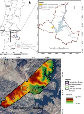
The study experimental site (farm “Herdade dos Gregos”), located in the surrounding area of the reservoir (Fig. 1), is a private property with 900 ha. The landscape is characterized by its hilly topography with significant altitude variations (mainly between 100 and 250 m). The bedrock of the study area is rocky, and, according to the World Reference Base for Soil Resources (FAO, 2006), the two types of soil in this area are Haplic Luvisols (LVha) and Lithic Leptosols (LPli). This farm was selected to include a diversity of land uses, including native montado grassland and more intensive land uses, with irrigation, namely olive tree orchard and lucerne cultivation. Direct pumping from Alqueva reservoir is done on this private property since it is near the reservoir.
The typical landscape in the Alentejo region is the mon-tado native grassland, an agrosilvopastoral system charac-terized by savannah-like, low-density woodlands with ever-green holm oaks (Quercus ilex). For that reason, an area of the montado grassland (20.7 ha), used as a permanent pas-ture for the cattle, was selected for this study. This small area is located in the high altitudes of the “Herdade dos Gre-gos” (from 200 to 240 m) with a slope that varies from 1.4 to 20.9 %. Tillage (at about 15 cm depths) was done only once every 10 years to decrease shrub competition (the most re-cent one was 4 years before the study implementation), and the soil is not subjected to any fertilizer. Four years before the study implementation, there was a fire on this agrosilvopas-toral area of the farm.
Taking advantage of the water availability, another land use (with 33.5 ha) is an irrigation area (pivot sprinkler irri-gation system) on which lucerne (Medicago sativa) is sown four times a year. Lucerne, once dried, is nutritional for
cat-Figure 1. Location of the study area at the Alqueva dam watershed
in Portugal.
tle, and it incorporates nitrogen in the soil. In this area, con-ventional tillage is used, involving multiple aspects: plough (about 20 cm depth) in fall, fallowing cultivator (about 15 cm depths) and disc harrow (about 10 cm depths) subsequent to soil tillage. Inorganic fertilizers were applied to the cultivated field at a rate of 100 kg NPK ha−1. This land use is placed in the midland (194–220 m), and the slope varies from 0 to 9 %. Another irrigated land use consists of an olive tree plan-tation (57.5 ha), which is done in strips. This cultivation has a drip irrigation system, is fertilized once every 2 years and is ploughed once a year to decrease weed competition. The olive orchard is located in the low elevations of the farm (150–186 m), and it is on the side of the reservoir (Fig. 1). The slope varies from 0 to 14.2 %.
2.2 Soil sampling and laboratory analysis
Since the objective was to study the relation between soil properties and the K factor from RUSLE, the soil samples were collected from 0 to 20 cm depth, according to Renard et al. (1997). In order to predict variations in short distances, 25, 27 and 52 soil samples were randomly collected respec-tively in montado, lucerne and the olive orchard (see Fig. 1).
Samples were air-dried and then dried for about 6 h at 40◦C on a ventilated oven, and they were passed through a 2 mm sieve to remove rocks and gravel. The particle-size distribu-tion was determined by the Bouyoucos hydrometer method (Bouyoucos, 1936). Soil organic matter content was deter-mined using the Walkley and Black (1934) method, a wet oxidation procedure. The soil’s total nitrogen content was determined according to Kjeldhal digestion, distillation and the titration method (Bremmer and Mulvaney, 1982). Soil pH and electrical conductivity were measured with a glass elec-trode in a 1 : 2.5 soil–water suspension (Watson and Brown, 2011).
2.3 Soil erodibility factor
Soil erodibility factor (K) (Mg ha h ha−1MJ−1mm−1)was estimated using soil property values – such as particle-size composition, content of organic matter, soil structure and permeability – in the 104 sample points described above. This factor represents the soil-loss rate per erosion index unit for a specified soil as measured on a standard plot (Renard et al., 1997). An algebraic approximation of the nomograph (Eq. 1) was used to estimate the K factor (Renard et al., 1997):
K = [2.1 × 10⁻⁴(12 − OM) × M1.14 (1)
+3.25(s − 2) + 2.5(p − 3)]/759,
where OM is the percentage of organic matter, s is soil struc-ture class, p is permeability class and M is the product of the percentage of modified silt (silt particles and very fine sand) or the 0.002–0.1 mm size fraction and the sum of the percentage of silt and percentage of sand. K is expressed in SI units of Mg ha h ha−1MJ−1mm−1. To estimate the perme-ability, the field-saturated hydraulic conductivity was mea-sured in the field using a double-ring infiltrometer (six site measurements per land use, each one with five repetitions). Permeability class and soil structure class were defined in ac-cordance with Renard et al. (1997).
2.4 Statistical and geostatistical analysis
Data were subjected to classical analysis using SPSS 17.0 software to obtain descriptive statistics, namely the mean, minimum and maximum; standard deviation (SD); coeffi-cient of variation (CV); and skewness of each parameter.
Soil data were introduced in the ArcGIS environment, and geostatistical analyses were performed using Geostatistical Analyst tool, in other to examine spatial distribution of soil properties. Prior to using geostatistics to obtain prediction maps, a preliminary analysis of data was done to check data normality and global directional trends. Skewness is the most common statistical parameter to identify a normal distribu-tion that is confirmed with skewness values varying form −1 to +1. Data transformation to normal distribution was nec-essary for some soil properties, and geostatistical analysis
tools were used (log or Box–Cox method). Trend analysis was performed to examine the presence of any global direc-tional trend in our data, an overriding process that affects all measurements in a deterministic way (nonrandom). So, when necessary, the trend removal was done using geosta-tistical analysis tools to more accurately model the variation (Panagopoulos et al., 2006).
The geostatistical methodology is based on the creation of a semivariogram (SV), a graphical representation (Eq. 2) that describes how samples are related to each other in space, and it is based on
γ (h) =1/2N (h) ×X[Zi−Z(i+h)]2, (2)
where γ (h) is the variance (the most related samples have lower values of variance), N (h) is the number of samples that can be grouped using vector h, Zirepresents the value of the sample and Zi+his the value of another sample located at a distance khk from the initial sample Zi (Chiles and Delfiner, 1999).
Ordinary Kriging (OK) was selected as a geostatistical method. OK is considered one of the most accurate interpo-lation techniques which assumes that variables close in space tend to be more similar than those further away (Goovaerts, 1999).
Using the Geostatistical Analyst tool (ArcGIS) and select-ing the OK methods, a semivariogram was created for each measured property. In the Kriging method different semivar-iogram models can be used (e.g., spherical, exponential) and the selection is usually performed by employing the cross-validation technique, which permits the evaluation of the pre-diction accuracy. Cross validation was executed to investi-gate the prediction performances through the statistical val-ues, as the mean error (ME) or root-mean-square standard-ized error (RMSSE), which results from comparing the es-timated semivariogram values and real observed values. Ad-ditional semivariogram parameters were analyzed to better understand the spatial structure and dependence of each vari-able. Nugget is the variance at distance zero and reflects the sampling error. Sill is the semivariance value at which the semivariogram reaches the upper bound and flattens out after its initial increase; it is the variance in which the samples are no longer spatially related to the study area.
Once the cross-validation process was completed, inter-polation maps of spatial distribution, for each soil variable, were produced according to the semivariogram model se-lected, in the ArcGIS software.
2.5 HJ-Biplot
HJ-Biplot represents a matrix, without assumptions related to its probabilistic distribution, permitting a graphic representa-tion of the geometric data structure, representing the data set (samples and variables) variability. The prefix “bi” is due to a simultaneous representation of the matrix rows and columns, searching for the maximum representation quality possible,
at the same scale (Martín-Rodríguez et al., 2002; González-Cabrera et al., 2006; Gallego-Álvarez et al., 2013).
A data matrix X suffers a factorization to reduce its dimen-sionality through single-value decomposition, the algebraic base of biplot representation (Gabriel, 1971):
X(n×p)=U(n×r)3(r×r)V0(r×p), (3) where 3(r×r)is a diagonal (λ1, λ2, . . ., λr) corresponding to the r eigenvalues of XX’ or XX0, U(n×r)is an orthogonal ma-trix whose columns are the eigenvectors of XX0or X0X and
U(n×r)is an orthogonal matrix whose columns are the eigen-vectors of XX0.
With the MultBiplot software, developed by the University of Salamanca (Vicente Villardón, 2014), an HJ-Biplot was used to determine the relation between soil properties and land uses, and the correlations between both (soil properties and land uses), thereby defining patterns and clustering the samples in groups.
On the HJ-Biplot graphic representation, the points repre-sent individuals (samples) and the vectors reprerepre-sent variables (in this case, chemical and physical soil properties). To inter-pret and discuss the graphs obtained with this methodology, it is essential to be aware of the following (Gallego-Álvarez et al., 2013):
– The distance between points represents the variability and can be interpreted as similarity or dissimilarity; i.e., the close samples have similar behaviors.
– The angle formed by variable vectors is interpreted as correlation; i.e., small angles between variables repre-sent similar behaviors with high positive correlations, and the obtuse angles that are almost a straight angle are associated with variables with high negative corre-lations; i.e., the cosine value of the angles represents the correlation between variables.
– The proximity of individual points and variable vectors means high preponderance; in other words the closer a point is to a variable vector, the more important this sample is to explain this variable.
– The length of the vector represents the variable’s vari-ability; the longer the vector, the higher this variability.
3 Results and discussion 3.1 Descriptive statistics
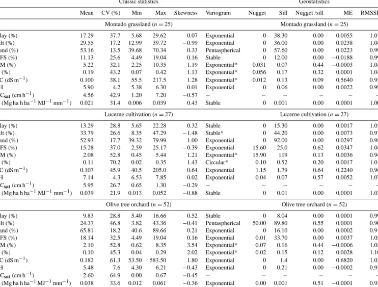
The descriptive statistics of soil properties are given in the first part of Table 1. All measured parameters varied consid-erably within the areas (different land uses) as indicated by the coefficient of variation (varies from 4.2 to 70.2 %). Ni-trogen (N) and organic matter (OM) show the highest vari-ation values, especially for cultivated fields (lucerne cultiva-tion and olive orchard), which can be explained with the lack
Table 1. Descriptive statistics of soil properties and parameters of the fitted variogram models and the cross-validation results.
Classic statistics Geostatistics
Mean CV (%) Min Max Skewness Variogram Nugget Sill Nugget /sill ME RMSSE
Montado grassland (n = 25) Montado grassland (n = 25)
Clay (%) 17.29 37.7 5.68 29.62 0.07 Exponential 0 38.30 0.00 0.0055 1.01 Silt (%) 29.55 17.2 12.99 39.72 −0.99 Exponential 0 36.00 0.00 0.0238 1.04 Sand (%) 53.16 13.5 39.68 70.34 0.33 Pentaspherical 0 57.60 0.00 0.0223 0.99 VFS (%) 11.13 25.6 4.49 19.04 0.16 Stable 0 12.00 0.00 −0.0188 0.99 OM (%) 5.22 32.1 2.25 10.35 1.19 Exponential* 0.031 0.07 0.44 −0.0003 1.04 N (%) 0.19 43.2 0.07 0.42 1.13 Exponential* 0.056 0.17 0.32 0.0001 1.04 EC (dS m−1) 0.100 38.1 55.5 217.5 1.28 Exponential* 0.012 0.13 0.09 0.5640 0.95 pH 5.90 4.2 5.38 6.30 0.01 Exponential 0 0.06 0.00 0.0022 0.99 HCsat(cm h−1) 4.56 42.9 1.20 7.20 −0.57 − − − − − − K (Mg ha h ha−1MJ−1mm−1) 0.021 31.4 0.006 0.039 0.43 Stable 0 0.001 0.00 0.0001 1.00
Lucerne cultivation (n = 27) Lucerne cultivation (n = 27)
Clay (%) 13.29 28.8 5.65 22.28 0.32 Stable 0 15.30 0.00 0.0017 1.02 Silt (%) 33.79 26.6 8.35 47.29 −1.48 Stable* 0 44.20 0.00 0.0073 0.97 Sand (%) 52.93 17.7 39.32 79.99 1.00 Exponential 0 92.00 0.00 0.0297 0.98 VFS (%) 15.28 37.0 2.59 25.17 −0.39 Exponential 15.60 25.0 0.62 0.0347 1.04 OM (%) 2.08 52.8 0.45 5.44 1.21 Exponential* 15.90 119 0.13 0.0036 0.94 N (%) 0.11 70.2 0.02 0.35 1.43 Circular* 0.10 0.52 0.20 0.0017 1.01 EC (dS m−1) 0.107 45.9 40.5 205.0 0.64 Exponential 1.15 1.79 0.64 0.2240 0.96 pH 7.14 4.3 6.53 7.85 0.02 Exponential 0.04 0.07 0.57 0.0052 1.07 HCsat(cm h−1) 5.95 26.7 0.65 1.30 −0.29 − − − − − − K (Mg ha h ha−1MJ−1mm−1) 0.039 21.9 0.013 0.052 −0.88 Stable 0 0.01 0.00 0.0001 1.03
Olive tree orchard (n = 52) Olive tree orchard (n = 52)
Clay (%) 9.83 28.8 5.40 16.66 0.52 Stable 0 8.04 0.00 0.0001 0.99 Silt (%) 24.37 46.8 3.82 43.36 −0.41 Pentaspherical 50.00 89.80 0.55 0.0001 0.90 Sand (%) 65.81 18.2 40.6 89.66 0.21 Exponential 0 16.10 0.00 0.0002 0.91 VFS (%) 18.14 32.5 4.49 19.04 0.16 Exponential 0.01 33.70 0.00 0.0037 1.05 OM (%) 2.10 52.8 0.62 8.35 3.54 Exponential* 0.07 0.16 0.44 −0.0006 1.02 N (%) 0.10 45.3 0.04 0.29 2.02 Exponential* 0.02 0.15 0.12 0.0028 1.10 EC (dS m−1) 0.182 61.3 53.50 583.50 1.80 Exponential 0 1.4 0.00 0.6820 1.02 pH 5.48 7.6 4.30 6.21 −0.43 Exponential 0 0.21 0.00 −0.0002 0.95 HCsat(cm h−1) 2.60 64.9 0.00 0.67 −0.45 − − − − − − K (Mg ha h ha−1MJ−1mm−1) 0.038 33.6 0.012 0.061 −0.36 Exponential 0.00 0.001 0.51 −0.0001 0.92
*Transformation for normal distribution.
CV – coefficient variation; Min – minimum; Max – maximum; VFS – very fine sand; N – nitrogen; OM – organic matter; EC – electrical conductivity; HCsat– saturated hydraulic conductivity; K – soil erodibility; ME – mean error; RMSSE – root-mean-square standardized error.
of homogeneous fertilization or tillage practices applied to soil in these areas.
The skewness results, which vary from −1.48 to 3.54 in this study, indicated that some soil properties of the differ-ent uses were not normally distributed, especially OM and N. The principal reason for some soil properties having non-normally distributions may be related to soil management practices (Tesfahunegn et al., 2011). As already mentioned, data were transformed to normal distribution when necessary (see Table 1).
These mean results show significant differences between land uses for all the properties analyzed. From the particle size distribution reported in Table 1, the soils are mostly sandy loam, formed mainly of sand, followed by silt and low quantities of clay. However, there are some differences be-tween land use areas that can be explained by soil type. The LPli soils are characterized by a thin layer (about 10 cm), in
that case upon a schist rock, justifying the higher clay content at the montado grassland. The LVha soils in the lucerne cul-tivation and the olive orchard are characterized by a loam or sandy loam layer (first 20 cm) with good drainage over clay-enriched subsoil (upon a basic crystalline rock), explaining the lower values of clay and fine sand, especially in the olive orchard. Despite the same soil type, soil texture is different between lucerne and the olive orchard, which can be justi-fied by land use. The lucerne is a more intensive cultivation (intensive irrigation, tillage and continuous cultivation; fer-tilizers and lime application), involving conditions that pro-mote changes in the soil weathering and moisture and, con-sequently, in soil texture (Yimer et al., 2008). On the other hand the soil between olive trees is kept without vegetation for most of the year and can explain the clay drainage to a sub-layer.
Montado shows the highest content of OM (5.22 %), whereas lucerne and olive fields show the lowest values (2.08 and 2.10 %, respectively). Other studies suggest that OM is higher in no-tillage soils compared to minimum tillage that increases aeration (Celik, 2005). Tillage mixes the sub-soil with topsub-soil; after sub-soil erosion, the nutrients are easily leached and the surface becomes poor in nutrients (Al-Kaisi and Licht, 2005). As for OM, the highest value of N nutri-ent occurs in the montado (0.19 %) and the lowest values in lucerne (0.11 %) and the olive orchard (0.10 %), which is re-lated to the tillage practice that is frequently employed in these last two land uses, while in the montado grassland the cattle enriches the soil.
Soil EC values (Table 1) were similar when comparing the montado grassland (0.100 dS cm−1) and the lucerne field (0.107 dS cm−1); they were slightly higher in the olive
or-chard (0.182 dS cm−1) but not enough to raise salinity
prob-lems. Usually, the addition of fertilizers (that happens on lucerne and the olive orchard) can cause high EC due to the percentage of the salts which are leached by water irrigation (higher in the lucerne field).
The soil pH was significantly higher in the lucerne culti-vation land (7.1) compared to the montado grassland (5.9) or in the olive tree orchard (5.5) (Table 1). The soil pH in the lucerne was greater due to lime application to increment the soil pH in that area. Lucerne’s optimum pH for production is between 6.5 and 7.2, and lime application has been found to produce a significant improvement in nodulation of lucerne (both number and dry weight of nodules per plant) (Grewal and Williams, 2001).
Saturated hydraulic conductivity (HC) values were greater in the lucerne area (5.95 cm h−1), slightly lower in the
mon-tado grassland (4.56 cm h−1) and lowest in the olive orchard
(2.60 cm h−1). The lower permeability in the olive orchard can be explained by the clay-enriched subsoil or soil crust problems, and it may explain the higher values of EC, i.e., the greater concentration of salts. Also it can be explained by the frequency of tillage in the different land uses because ag-gregate stability and water infiltration rate are higher in soils subjected to limited tillage systems (Alvarez and Steinbach, 2009).
As a result, the K factor was different for the typical land use, montado grassland, compared to the lucerne cultivation and the olive orchard. The values increased with the inten-sification of the cultivation field, with the lowest values for montado grassland (0.021 Mg ha h ha−1 MJ−1mm−1) and
the highest for the lucerne cultivation (0.039 Mg ha h ha−1
MJ−1mm−1) and the olive orchard (0.038 Mg ha h ha−1
MJ−1mm−1). Other studies had similar results, showing that the removal of permanent vegetation, the loss of OM and the reduction of aggregation, caused by intensive cultivation, contribute to decrease the K factor (Celik, 2005).
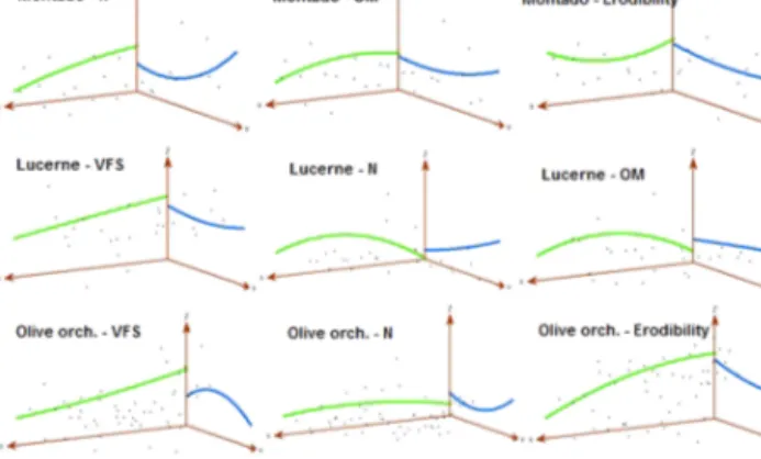
Figure 2. Three-dimensional perspective of the trends in the input
data sets.
3.2 Spatial dependence of soil properties
Model selection for each soil property was based on the nugget, sill, ME and the RMSSE presented in the second part of Table 1 (Geostatistics).
Nugget is low in most soil properties studied, implying strong spatial dependence. The nugget-to-sill ratio is used to define spatial dependence of soil properties: if the ratio is < 0.25, there is strong spatial dependence; if it is 0.25 to 0.75, there is moderate spatial dependence; and if the ratio is > 0.75, spatial dependence is weak (Cambardella et al., 1994). As shown in Table 1 the ratio values indicate the pres-ence of high to moderate spatial dependpres-ence for all soil pa-rameters (values between 0 and 0.64). In general, there is stronger spatial dependence in montado (low nugget-to-sill ratio), which can be explained with the non-existence of ex-trinsic factors, such as management cultivation practices, that influence soil properties, and soil is left as it is for permanent pasture.
Cross validation facilitated the selection of the best-fit semivariogram for an interpolation map, which could pro-vide the most accurate predictions. Closer values of the ME to 0, and closer values of the RMSS to 1, suggested that the prediction values were close to measured values (Wackker-nagel, 1995). Most of the soil properties were best fitted with an exponential model, particularly in the montado area and olive orchard, whereas in lucerne the Gaussian, circular and stable semivariogram models were used.
3.3 Spatial distribution
The interpolation maps obtained with geostatistics are useful to better understand spatial variability and its influences. The variability of spatial soil properties can be influenced by nat-ural factors (such as particle-size composition and topogra-phy) and anthropogenic factors (such as land cover or man-agement practices) (Tesfahunegn et al., 2011). Sometimes, the effect of some factors is at least 1 order of magnitude
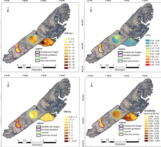
Figure 3. Prediction map of very fine sand (VFS), total nitrogen (N), organic matter (OM) and soil erodibility (K factor).
greater (as topography or soil type) than the land use. So, as mentioned trend analysis was performed to study the exis-tence of directional trends caused by these factors with large scale of variation, and it is shown in Fig. 2. Global trend ex-ists if a curve that is not flat (i.e., a polynomial equation) can be fitted to the data (for example for total N in montado or very fine sand (VFS) in the olive orchard). These trends were identified for part of the soil properties and for differ-ent land uses (Fig. 2). The strongest influence of a directional trend was identified from southeast to the northwest, which could be associated with the topography (Fig. 1) since the al-titudes increase in accordance with these direction. So, trend removal is crucial to create more accurate prediction maps in order to justify an assumption of normality.
The interpolation maps for some studied soil properties are shown in Fig. 3. Through looking at the VFS distribu-tion, it was noticed that the higher fractions of these particles (Fig. 3) were measured at low altitudes or on flat slopes such as the valley (see elevation in Fig. 1). This can be explained by erosion–deposition processes because these particles are easily detached and transported by water.
The highest percentages of N and OM were found on mon-tado, as discussed previously. These two properties present
similar distributions for all land uses. The nitrogen existing in the soil is mostly organic, and the inorganic forms (ammo-nium and nitrate) are easily leached or assimilated by plants. So, when OM breaks down due to mineralization, the N frac-tion decreases (Varennes, 2003). There were higher values in montado because the soil is not frequently tilled as it is in the other land uses. In the lucerne cultivation and the olive or-chard, the variation of OM and N can be explained by inad-equate management practices (e.g., inadinad-equate fertilization rates, tillage, irrigation rates, seed rates).
Figure 3 illustrates the interpolation map for the K fac-tor which was estimated through the Wischmeier nomograph (Eq. 1). The values vary from 0.006 to 0.061 Mg ha h ha−1 MJ−1mm−1, and the prediction map shows the highest val-ues for lucerne and the olive orchard, especially where the soils have more silt and VFS, along with less OM and N (see HJ-Biplot). In the surrounding area of the reservoir, the types of soil differ with the topography and land use; therefore, knowledge of soil properties is fundamental when facing the intensification of cultivation that could increase the K factor. These intensive practices decrease OM in soils, making them poor and vulnerable to the soil erosion process.
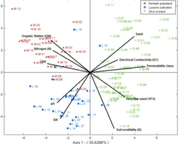
Figure 4. The HJ-Biplot representation matrix of soil samples and
studied variables.
When looking for natural vs. anthropogenic impact on the
K factor, for each land use, it is evident that in the montado the spatial variability is mainly associated with natural (in-trinsic) factors (as texture), with soil properties and erodibil-ity distribution being more homogenous. In the lucerne and olive orchard the spatial variability is more dependent on in-homogeneous anthropogenic causes such as fertilization and irrigation rates and tillage/plough processes.
3.4 HJ-Biplot
The HJ-Biplot representation matrix of soil properties is showed in Fig. 4. It was observed that the dominant axis (axis 1) takes 35.83 % of the total inertia (information) of the system. With both dimensions, an accumulative inertia of 61.04 % was achieved. Regarding this graphic representa-tion, it was observed that samples were grouped according to the land use. The montado samples were close to OM, N and clay vectors, showing their preponderance to be a character-ization of these variables. The lucerne samples were impor-tant to describe the pH and silt content. On the other hand the olive samples were more disperse but related to EC, perme-ability class, sand, VFS and K.
The variables demonstrating a more positive correlation were OM and N, as previously noticed. Clay and silt were also positively correlated, but they were negatively correlated with sand, as expected, because soils with more sand have less clay and/or silt.
Through the matrix representation it was detected that soils with more sand have higher EC (olive orchard), al-though EC normally increases with the percentage of clay. This may be explained by the addition of fertilizers, as previ-ously discussed, that can contribute to an EC increase. These results for EC show low variability between land uses, reveal-ing a low cation exchange capacity of these soils. This is
fre-Figure 5. Hierarchical clusters representation of soil samples and
studied variables.
quently caused by intensive soil mobilization (Paz-González et al., 2000).
Permeability class increases as the HCsatdecreases, as
de-fined by Renard et al. (1997). So, contrary to what was ex-pected, for this study the soils with more sand (occurring in the olive orchard) have less hydraulic conductivity (high-permeability class). It can be explained by a clay-enriched sub-layer under the sandy loam layer or/and by the soil compaction/degradation processes. The soil compaction and degradation can be related to repeated plow operations to re-duce shrubs between olive rows and irrigation (Pagliai et al., 2004). This permeability decrease in the olive orchard was correlated with the increase of the K factor.
Nevertheless, the properties more positively correlated with the K factor were the VFS and silt; this is due to the susceptibility of these particles to erosion since they can be easily detached and transported by water (Morgan, 2005). The OM and N content were negatively correlated with K and permeability. The higher OM reduces the susceptibility of the soil to detachment and increases infiltration (Bronick and Lal, 2005). The N content is not used to estimate K; however, especially for soils without fertilization, the exis-tent N is mostly associated with OM. Nevertheless, nutrients decrease in soils that are more erodible, according to the liter-ature (Tesfahunegn et al., 2011). The clay content also shows a negative correlation with K factor, as expected (Renard et al., 1997).
Figure 5 shows the hierarchical cluster representation. Us-ing HJ-Biplot methodology and the aggregation tool ward, three clusters were obtained. The samples were grouped by land uses (that were already detected by the matrix represen-tation; see Fig. 4). Cluster 1 is represented by a majority of samples from lucerne, Cluster 2 by samples from montado and Cluster 3 by samples from the olive orchard. This was
explained by the effect of different management practices, vegetation cover and local soil characteristics, as discussed. Some samples in each land use had different values (higher or lower than the majority) and were grouped in a different cluster. Identifying the location of the sample, the cause of displacement can be studied and can help to improve land management practices.
Therefore, the cluster analysis is convenient to identify the effect of different land use and management on soil prop-erties and consequently on soil erosion. On the other hand, the cluster analysis could support the delineation of zones according to soil properties, and subsequently according to erosion susceptibility, which could be used for site-specific soil management recommendations.
4 Conclusions
This study demonstrated that the variability of soil proper-ties and the K factor is associated with land use, cultural practices (tillage type, fertilizer rates, conservation measures, etc.) and local conditions (complex topographic landscape, soil type, etc.). The K factor showed high correlation espe-cially with organic matter, nitrogen, silt and very fine sand. Soils with intensively cultivated land use, and consequently with more tillage and irrigation, had lower organic matter and lower nitrogen content. This translates into a lower cation exchange capacity producing lower aggregate stability and, consequently, an increase of the K factor.
Therefore, in the surrounding area of the Alqueva reser-voir, the ongoing change in land use and soil management practices can have a significant effect on chemical and physi-cal soil properties. As a result, this affects the soil erodibility index, intensifying the risk of erosion. The increase of soil loss in the watershed might have a significant impact on a reservoir’s ability to store water, reducing its lifespan.
Knowledge of soil spatial variability is fundamental for environment management and can help in the sustainable use of the resource soil. The prediction maps produced with geo-statistics are an important monitoring tool, showing the exact position in the field of the specific soil properties. The HJ-Biplot methodology was demonstrated to be useful in gain-ing a better understandgain-ing of how soils properties were cor-related and allowed not only a determination of the behav-ior by sample but also a conclusion as to which variable is responsible for such behavior. The simultaneous use of HJ-Biplot with geostatistics allows this information to be found on the map, which has important theoretical and practical significance for precision agriculture. Facing the intensifica-tion of cultivaintensifica-tion in the surrounding area of the reservoir, site-specific soil management and careful land use planning are needed to take into account the spatial variability of soil properties, delineating management zones, variable fertiliza-tion management, irrigafertiliza-tion scheduling, conservafertiliza-tion prac-tices and other efforts.
Acknowledgements. The authors want to thank the Portuguese Foundation for Science and Technology for its support in this research project (PTDC/AAC-AMB/102173/2008 and SFRH/BD/69548/2010) and the Research Center for Spatial and Organizational Dynamics (CIEO) for having provided the conditions to publish this work.
Edited by: A. Cerdà
References
Al-Kaisi, M. M. and Lichtm, M. A.: Soil carbon and nitrogen changes as influenced by tillage and cropping systems in some Iowa soils, Agric. Ecos. Environ., 105, 635–647, 2005.
Alvarez, R. and Steinbach, H. S.: A review of the effects of tillage systems on some soil physical properties, water content, nitrate availability and crops yield in the Argentine Pampas, Soil Till. Res., 104, 1–15, 2009.
Biro, K., Pradhan, B., Buchroithner, M., and Makeschin, F.: Land use/land cover change analysis and its impact on soil proper-ties in the Northern part of Gadarif region, Sudan, Land Degrad. Dev., 24, 90–102, 2013.
Blavet, D., De Noni, G., Le Bissonnais, Y., Leonard, M., Maillo, L., Laurent, J. Y., Asseline, J., Leprun, J. C., Arshad. M. A., and Roose, E.: Effect of land use and management on the early stages of soil water erosion in French Mediterranean vineyards, Soil Till. Res., 106, 124–136, 2009.
Bouyoucos, G.: Directions for making mechanical analysis of soils by the hydrometer method, Soil Sci., 42, 225–228, 1936. Bremmer, J. and Mulvaney, C.: Nitrogen-total, in: Methods of Soil
Analysis Part 2, Chemical and Microbiological Properties, edited by: Page, A. L., Miller, R. H., and Keeney, D. R., Soil Science Society of America, Madison, WI, USA, 595–625, 1982. Bronick, C. J. and Lal, R.: Soil structure and management: a review,
Geoderma, 124, 3–22, 2005.
Cambardella, C. A., Moorman, T. B., Novak, J. M., Parkin, T. B., Karlen, D. L., Turco, R. F., and Konopka, A. E.: Field-scale vari-ability of soil properties in Central Iowa soils, Soil Sci. Soc. Am. J., 58, 1501–1511, 1994.
Celik, I.: Land-use effects on organic matter and physical properties of soil in a southern Mediterranean highland of Turkey, Soil Till. Res., 83, 270–277, 2005.
Cerdà, A. and Doerr, S. H.: Soil wettability, runoff and erodibility of major dry-Mediterranean land use types on calcareous soils, Hydrol. Process., 21, 2325–2336, 2007.
Cerdà, A., Giménez-Morera, A., and Bodí, M. B.: Soil and water losses from new citrus orchards growing on sloped soils in the western Mediterranean basin, Earth Surf. Proc. Land., 34, 1822– 1830, 2009.
Chiles, J. P. and Delfiner, P.: Geostatistics: Modelling Spatial Un-certainty, John Wiley & Sons, New York, 1999.
FAO: World reference base for soil resources. A framework for in-ternational classification, correlation and communication, World Soil Resources Reports 103, Rome, 2006.
Gabriel, K. R.: The biplot graphic display of matrices with applica-tion to principal component analysis, Biometrika, 58, 453–467, 1971.
Gallego-Álvarez, I., Rodríguez-Domínguez, L., and García-Rubio, R.: Analysis of the environmental issues worldwide: a study from the biplot perspective, J. Clean. Prod., 42, 19–30, 2013.
Garcia-Talegon, J., Vicente, M. A., Molina-Ballesteros, E., and Vicente-Tavera, S.: Determination of the origin and evolution of building stones as a function of their chemical composition us-ing the inertia criterion based on an HJ-biplot, Chem. Geol., 153, 37–51, 1999.
González-Cabrera, J., Hidalgo-Martínez, M., Martín-Mateos, E., and Vicente-Tavera, S.: Study of the evolution of air pollution in Salamanca (Spain) along a five-year period (1994–1998) using HJ-Biplot simultaneous representation analysis, Environ. Model. Softw., 21, 61–68, 2006.
Goovaerts, P.: Geostatistics for Natural Resources Evaluation, Ox-ford University Press, New York, 1997.
Grewal, H. and Williams, R.: Lucerne varieties differ in their re-sponse to liming on an acid soil, in: The date of the conference is: Proceedings of the 10th Australian Agronomy Conference, Hobart, Tasmania, 29 January to 1 February 2001, Australian So-ciety of Agronomy, 92–95, 2001.
Haregeweyn, N., Poesen, J., Verstraeten, G., Govers, G., de Vente, J., Nyssen, J., Deckers, J., and Moeyersons, J.: Assessing the performance of a spatially distributed soil erosion and sed-iment delivery model (WATEM/SEDEM in Northern Ethiopia, Land Degrad. Dev., 24, 188–204, 2013.
Lal, R.: Soil degradation by erosion, Land Degrad. Dev., 12, 519– 539, 2001.
Leh, M., Bajwa, S., and Chaubey, I.: Impact of land use change on erosion risk: and integrated remote sensing geopraphic informa-tion system and modeling methodology, Land Degrad. Dev., 24, 409–421, 2013.
Lopez-Bermudez, F., Romero-Diaz, A., and Martinez-Fernandez, J.: Vegetation and soil erosion under a semi-arid Mediterranean climate: a case study from Murcia (Spain), Geomorphology, 24, 51–58, 1998.
Mandal, D. and Sharda, V. N.: Appraisal of soil erosion risk in the Eastern Himalayan region of India for soil conservation plan-ning, Land Degrad. Dev., 24, 430–437, 2013.
Martín-Rodríguez, J., Galindo-Villardón, P., Vicente-Villardón, J. L.: Comparison and integration of subspaces from a biplot perspective, J. Stat. Plan. Infer., 102, 411–423, 2002.
Morgan, R. P. C.: Soil Erosion and Conservation, Blackwell Pub-lishing, Oxford, 2005.
Nunes, J. P., Seixas, J., Keizer, J. J., and Ferreira, A. J. D.: Sensitiv-ity of runoff and soil erosion to climate change in two Mediter-ranean watersheds: Part I. Model parameterization and evalua-tion, Hydrol. Process., 23, 1202–1211, 2009.
Pagliai, M., Vignozzi, N., and Pellegrini, S.: Soil structure and the effect of management practices, Soil Till. Res., 79, 131–143, 2004.
Panagopoulos, T. and Antunes, M. D. C.: Integrating geostatistics and GIS for assessment of erosion risk on low density Quercus suber woodlands of South Portugal, Arid Land Res. Manag., 22, 159–177, 2008.
Panagopoulos, T., Jesus, J., Antunes, M. D. C., Beltrao, J.: Analysis of spatial interpolation for optimising management of a salinized field cultivated with lettuce, Eur. J. Agron., 24, 1–10, 2006.
Panagopoulos, T., Jesus, J., Blumberg, D., and Ben-Asher, J.: Spa-tial variability of wheat yield as related to soil parameters in an organic field, Comm. Soil Sci. Plant Anal., 45, 2018–2031, 2014. Pandey, A., Chowdary, V. M., and Mal. B. C.: Identification of critical erosion prone in the small agricultural watershed using USLE, GIS and remote sensing, Water Resour. Manag., 21, 729– 746, 2007.
Paz-González, A. V. S., Vieira, S. R., and Castro, M. T.: The effect of cultivation on spatial variability of selected properties of an umbric horizon, Geoderma, 97, 273–292, 2000.
Pérez-Rodríguez, R., Marques, M., and Bienes, R.: Spatial variabil-ity of the soil erodibilvariabil-ity parameters and their reaction with the soil map at subgroup level, Sci. Total Environ., 378, 166–173, 2007.
Renard, K. G., Foster, G. R., Weesies, G. A., McCool, D. K., and Yoder, D. C.: A Guide to Conservation Planning with the Revised Universal Soil Loss Equation (RUSLE). Agricultural Handbook No 703, United States Department of Agriculture, Agricultural Regional Service, Washington DC, 1997.
Tesfahunegn, G. B., Tamene, L., and Vlek, P. L. G.: Catchment-scale spatial variability of soil properties and implications on site-specific soil management in northern Ethiopia, Soil Till. Res., 117, 124–139, 2011.
Varennes, A.: Produtividade dos solos e Ambiente, Escolar Editora, Lisbon, Portugal, 2003.
Vicente-Villardón, J.: MULTBIPLOT: a package for Multivariate Analysis using Biplot, Departamento de Estadística, Universidad de Salamanca, Salamanca, 2014.
Wackernagel, H.: Multivariate Geostatistics: an Introduction With Applications, Springer, Berlin, 1995.
Walkley, A. and Black, I. A.: An examination of Degtjareff method for determining soil organic matter and a proposed modification of the chromic acid titration method, Soil Sci., 37, 29–37, 1934. Wang, Y. Q. and Shao, M. A.: Spatial variability of soil physical properties in a region of the loess plateau of PR China subject to wind and water erosion, Land Degrad. Dev., 24, 296–304, 2013. Watson, M. E. and Brown, J. R. (Ed.): pH and lime requirement, in: Recommended Chemical Soil Test Procedures for the North Cen-tral Region, North CenCen-tral Regional Research Publication Num-ber 22, Agricultural Experiment Station SB 1001, Columbia, Missouri, USA, 13–16, 1998.
Yang, D., Kanae, S., Oki, T., Koikel, T., Musiake, T.: Global poten-tial soil erosion with reference to land use and climate change, Hydrol. Process., 17, 2913–2928, 2003.
Yimer, F., Ledin, S., and Abdelkadir, A.: Concentrations of ex-changeable bases and cation exchange capacity in soils of crop-land, grazing and forest in the Bale Mountains, Ethiopia, Forest Ecol. Manag., 256, 1298–1302, 2008.
Zhao, G., Mu, X., Wen, Z., Wang, F., and Gao, P.: Soil erosion, conservation, and eco-environment changes in the Loess Plateau of China, Land Degrad. Dev., 24, 499–510, 2013.
Ziadat, F. M. and Taimeh, A. Y.: Effect of rainfall intensity, slope and land use and antecedent soil moisture on soil erosion in an arid environment, Land Degrad. Dev., 24, 582–590, 2013.