Heat sources within the Greenland Ice Sheet: dissipation, temperate paleo-firn and cryo-hydrologic warming

(1)

www.the-cryosphere.net/9/245/2015/ doi:10.5194/tc-9-245-2015

Heat sources within the Greenland Ice Sheet: dissipation, temperate

paleo-firn and cryo-hydrologic warming

M. P. Lüthi1,*, C. Ryser1, L. C. Andrews2,3, G. A. Catania2,3, M. Funk1, R. L. Hawley4, M. J. Hoffman5, and T. A. Neumann6

1_{Versuchsanstalt für Wasserbau, Hydrologie und Glaziologie (VAW), ETH Zurich, 8093 Zurich, Switzerland} 2_{Institute for Geophysics, The University of Texas at Austin, Austin, Texas, 78758, USA}

3_{Dept. of Geological Sciences, The University of Texas at Austin, Austin, Texas, 78713, USA} 4_{Dept. of Earth Sciences, Dartmouth College, Hanover, New Hampshire, 03755, USA}

5_{Fluid Dynamics and Solid Mechanics Group, Los Alamos National Laboratory, Los Alamos, New Mexico, 87545, USA} 6_{NASA Goddard Space Flight Center, Code 615, Greenbelt, Maryland, 20770, USA}

*_{now at: Geographical Institute, University of Zurich, 8057 Zurich, Switzerland}

Correspondence to:M. P. Lüthi ([email protected])

Received: 24 September 2014 – Published in The Cryosphere Discuss.: 13 October 2014 Revised: 22 December 2014 – Accepted: 20 January 2015 – Published: 9 February 2015

Abstract. Ice temperature profiles from the Greenland Ice Sheet contain information on the deformation history, past climates and recent warming. We present full-depth tem-perature profiles from two drill sites on a flow line passing through Swiss Camp, West Greenland. Numerical modeling reveals that ice temperatures are considerably higher than would be expected from heat diffusion and dissipation alone. The possible causes for this extra heat are evaluated using a Lagrangian heat flow model. The model results reveal that the observations can be explained with a combination of dif-ferent processes: enhanced dissipation (strain heating) in ice-age ice, temperate paleo-firn, and cryo-hydrologic warming in deep crevasses.

1 Introduction

Vertical ice temperature profiles of the Greenland Ice Sheet (GrIS) carry information on past upstream surface temper-ature and accumulation rates. This information is modi-fied by vertical and horizontal stretching of the ice during flow, smoothed by diffusion, and altered by subglacial and englacial heat sources.

Characteristic ideal profiles at different locations in the ice sheet have been obtained with numerical advection-diffusion models (e.g., Budd et al., 1982; Letreguilly et al., 1991; Funk

et al., 1994; Greve, 1997). Full-depth ice temperature profiles from the ablation zone of the GrIS have been published for only nine drill sites: five in the ablation zone of the Paakit-soq area, downstream of Swiss Camp (Thomsen et al., 1991) and four in Jakobshavn Isbræ (Iken et al., 1993; Lüthi et al., 2002). Despite the limited spatial extent of these observa-tions, comparison between modeled and observed temper-ature profiles allow us to explore the complexity of heat sources in the ablation zone.

(2)

Figure 1.The study site indicated with red area within Greenland outline is illustrated with a MODIS satellite image provided by NASA/GSFC (2010). The drill sites FOXX and GULL are located on a flow line downstream of Swiss Camp, and north of Jakovshavn Isbræ. Site DUCK is from 1995 (Lüthi et al., 2002). Drill sites by Thomsen are marked with yellow triangles and indicated by TD1-5. The inset shows bed and surface topographies along the flow line at 5-fold vertical exaggeration (data from DTU Space and Re-mote Sensing, 2005; Gogineni, 2012).

as “cryo-hydrologic warming” (Phillips et al., 2010, 2013). Future increases in melt area extent might therefore lead to more cryo-hydrologic warming, a mechanism considered to cause rapid future warming of the ice sheet (Phillips et al., 2013).

In this study we present full-thickness temperature pro-files from four new boreholes. Using a numerical heat flow model we calculate expected ice temperature profiles for our study sites. Comparison of modeled profiles with measure-ments shows warmer temperatures of the ice in the ablation area. Possible sources of this extra heat are investigated and discussed.

2 Data and methods 2.1 Drill sites

The location of the three drill sites in the western abla-tion zone of the GrIS is indicated on the map in Fig. 1. Sites FOXX and GULL were instrumented in summer 2011 with sensors for ice deformation, subglacial pressure, and ice temperature (Ryser et al., 2014a, b; Andrews et al., 2014). Deep drilling at Swiss Camp and installation of thermistor string TD5 in 1990 was performed by Danish Technological University (DTU; Thomsen and Thorning, 1992; Ahlstrom, 2007).

2.2 Temperature measurements

At sites FOXX and GULL temperature was measured with the custom-built digital borehole sensor system DIBOSS (described in Ryser et al., 2014b) at depths below 300 m. These deep sensors are complemented with analog thermis-tors closer to the surface. In each DIBOSS sensing unit an IST TSic-716 semiconductor temperature sensor with inte-grated 14 Bit AD-converter (resolution 4 mK,±70 mK abso-lute) was mounted in direct contact with the enclosing alu-minum housing. These sensors were logged in 10 min inter-vals for 2 years with a Campbell CR-1000 data logger. De-pending on ambient ice temperature, the readings of tempera-ture equilibrated to their undisturbed values after one to three months.

For measurements close to the surface, sets of two ther-mistor strings were deployed in two boreholes at site FOXX, and in one borehole at site GULL. Each string consisted of an 18-core cable with 9 NTC thermistors (Fenwal 135-103FAG-J01) that were shielded from pressure and moisture, and for which individual calibration curves were determined in a cal-ibration bath at six to eight reference temperatures in the range of−17.5 to 10◦C with a digital multi-meter. Refer-ence thermistors, calibrated to an absolute accuracy of 20 mK by the Swiss Federal Office of Metrology, were used to de-termine the bath temperature. The maximum difference be-tween reference temperatures and the calibration curve was 40 mK. In the field, resistances were measured with a full bridge circuit logged by a Campbell CR-1000 data logger, and occasional readings with a digital multi-meter over the course of 2 years. With the setup described above, the abso-lute accuracy of all measured temperatures is estimated to be better than 70 mK.

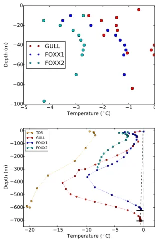
Figure 2 shows ice temperature measured at sites FOXX, GULL and TD5 (Swiss Camp; Thomsen and Thorning, 1992). Ice temperature increases from the highest site to-wards the margin. A notable exception is profile FOXX2 which was recorded in 86 m distance from FOXX1, and which is even colder than GULL.

2.3 Heat sources

Heat sources within the ice are due to dissipation (strain heat-ing), or related to flowing or freezing water. Here we calcu-late order of magnitude estimates of these effects. For this purpose we assume ice with a density ofρi=900 kg m−3,

heat capacity Ci=2093 J kg−1 and latent heat of freezing

(3)

2.3.1 Freezing water

The heat energy from freezing water needed to raise the tem-perature of 1 m3of ice by1T =1 K is

W =ρiCi1T =1.88 MJ m−3. (1)

To produce this amount of heat by freezing, 5.6 kg of water are required. Such water is readily available at the glacier sur-face during the ablation season, and also in the lower reaches of the accumulation area where permanent storage of wa-ter within the firn was recently discovered, although 250 km south of our sites (e.g., Harper et al., 2012; Forster et al., 2013). Water seeping through cracks can freeze and provide an extensive heat source down to the bottom of such cracks. 2.3.2 Strain heating

The volumetric heat production rate P due to dissipation (strain heating) under shear deformation is calculated under the assumption of the shallow ice approximation and n=3 as

P = ˙εijσij∼2ε˙xzσxz=2A(T )σxz4, (2)

where the shear stress σxz=ρig htanαis calculated from

the density ρi, gravityg, surface slope α and depth h

be-low the surface. The value of P therefore varies with cur-rent surface slope, and depends on depth and curcur-rent tem-perature. The temperature dependent flow rate factor A(T )

is taken from Cuffey and Paterson (2010) which agrees well with measurements of ice deformation at sites FOXX and GULL (Ryser et al., 2014b). At a shear stress of 0.1 MPa and withA(−5◦C)=29.3 MPa−3a−1the heating power is

P =0.006 MJ m−3a−1, equivalent to a heating rate of 0.31 K per century.

2.4 Heat flow model

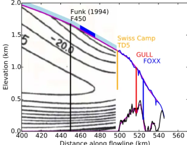
The heat flow model is adapted to model the lower accumu-lation and upper abaccumu-lation areas in our region of study. The model tracks a flowline with origin at the ice sheet center (0 km; Fig. 7b in Funk et al., 1994). Figure 3 shows our area of interest, located on this flow line between coordinate 450 and 530 km. In this coordinate system, the 1990 drill site TD5 (Thomsen et al., 1991) at Swiss Camp is located at co-ordinate 498 km at the equilibrium line. The two 2011 drill sites FOXX and GULL are located at coordinates 520 and 530 km.

Heat flow is modeled with the finite element method in two dimensions. The model implements a block of ice in Lagrangian description. The finite element library Libmesh (Kirk et al., 2006) was used to solve the transient heat diffu-sion equation in a Lagrangian reference frame (i.e., the mesh nodes follow the deforming material; e.g., Hutter and Jöhnk, 2004)

5 4 3 2 1 0

Temperature (◦C)

100 80 60 40 20 0

Depth (m)

GULL

FOXX1

FOXX2

20 15 10 5 0

Temperature (◦C)

700 600 500 400 300 200 100 0

Depth (m)

TD5 GULL FOXX1 FOXX2

Figure 2.Measured ice temperatures.(a)shows near-surface tem-peratures at sites GULL and FOXX. Holes FOXX1 and FOXX2 are 86 m apart.(b)shows measured ice temperatures in four boreholes at the drill sites TD5 (Swiss Camp; data from Thomsen et al., 1991), GULL and FOXX. The dashed line indicates the pressure melting temperature.

ρiCi

∂T

∂t = ∇(k∇T )+P , (3)

with temperatureT, densityρi, specific heat capacityCi, heat

conductivityk and volumetric heat production rate P. The model domain consists of a block discretized with rectangu-lar Quad4 elements with Galerkin weighting (linear approx-imation of temperature). Implicit time stepping was imple-mented with a standard Crank–Nicolson scheme.

Each model run consisted of the deformation of the block of ice (the model domain) during horizontal motion over the distance of 100 km (from 450 to 550 km; Fig. 3). The hori-zontal velocity was taken from Funk et al. (1994), resulting in a travel time from Swiss Camp to FOXX of∼900 years. During motion along the flow line the model domain (the block) is horizontally and vertically stretched or compressed to comply with the local ice thickness. Vertical shearing was neglected (i.e., ε˙xz=0) so that the block moved in

(4)

Table 1. Designation of model runs with different heat sources. These sources are combined in different model runs, e.g., run mEC.

mC refreezing of water-filled crevasses

mD dissipation from strain heating/reference run mE dissipation from strain heating with enhancement mF temperate firn above equilibrium line

withε˙zz= −˙εxx andε˙yy=0 (with coordinatesx in flow

di-rection,yacross,zvertical). Nodes were moved according to their position with respect to the origin of the coordinate sys-tem of the Lagrangian model domain. Heat (i.e., sys-temperature at the model nodes as the solution from an earlier time step) is therefore advected with the mesh in horizontal and vertical direction.

Mass accumulation at the upper surface was simulated by adding new elements on top of the domain, in which temper-ature was set to the surface tempertemper-ature. Surface tempertemper-ature and mass balance are taken from Fig. 4 in Funk et al. (1994), which are similar to the 1900–2000 values of a more recent reconstruction (Box, 2013). Similarly, mass removal by sur-face melt was implemented by removing elements from the top of the domain. In the Libmesh implementation this was achieved in a simple manner by solving the heat flow equa-tion in a subdomain of a larger mesh with constant topology. With this approach, only the extent of the active subdomain was adjusted in every time step. To obtain a high resolution of the grid close to the surface the mesh was refined to a res-olution of 0.5 m in the top 150 m of the active subdomain, using the adaptive mesh refinement with hanging nodes im-plemented in Libmesh, as illustrated in Fig. 4. The unrefined mesh consisted of 100 elements in the vertical, correspond-ing to a vertical mesh size of 20 to 7 m, dependcorrespond-ing on total ice column height. A constant time step size of 1 year was used, which together with the vertical mesh size of 0.5 m at the surface gives a numerically stable solution. This model setup closely reproduced analytical solutions for two setups: Sinusoidal forcing of the surface temperature, and a mov-ing boundary solution for constant surface ablation (Vorkauf, 2014).

The initial dimensions of the model domain were 1000 m length and 2000 m thickness. The mesh was refined around the vertical coordinate 1670 m corresponding to the vertical position of the initial surface. Elements above the current sur-face were flagged to belong to the inactive subdomain. The heat flow Eq. (3) was solved in the active subdomain below the surface, with Dirichlet boundary conditions (prescribed temperature) at the uppermost active element, and melting point temperature at the bottom. On the upstream and down-stream faces a zero-flux boundary condition was prescribed. Figure 4 illustrates the progressive deformation of the mesh, the refinement of elements around the surface, and the vary-ing number and extent of active elements. In all model runs the mesh was considerably finer than shown in Fig. 4; 200

el-400 420 440 460 480 500 520 540 560

Distance along flowline (km)

0.0

0.5

1.0

1.5

2.0 Elevation (km)

Funk (1994)

F450

Swiss Camp

TD5

GULL

_FOXX

Figure 3.The locations and depths of temperature profiles at sites TD5, GULL and FOXX are shown as colored vertical lines on a background plot of the modeled temperature field from Fig. 7b in Funk et al. (1994). The temperature profile F450 at horizontal coor-dinate 450 km is used as model input. Bedrock (black) and surface (blue) was obtained from radar data (Gogineni, 2012). Smoothed versions, indicated with purple lines, were used as model input. The light blue area indicates cold firn conditions, and the dark blue area between 460 and 475 km the area within which the temperate firn that emerges at TD5 was accumulated between 1570 and 1730.

ements in the vertical, 20 in the horizontal, and the mesh was refined around the surface in 5 steps instead of the 3 steps displayed in the figure for illustration.

The initial temperature profile F450, located 450 km along the flow line, is taken from Funk et al. (1994, Fig. 8b). This profile was obtained by solving the advection-diffusion equa-tion with a discrete phase-change boundary along the flow line from the ice sheet center, with prescribed surface and basal velocity. In our model, the block is assumed to move at prescribed horizontal velocities, also taken from Fig. 4 in Funk et al. (1994). These velocities are similar to those from recent satellite imagery feature tracking (Joughin et al., 2008).

3 Model results

In the following we compare model runs of the heat flow model with borehole data. The model runs are driven with different internal heat sources, and a modified surface bound-ary condition. These assumptions are independent from each other, and are combined to investigate the origin of mea-sured temperatures profiles. Designations of model runs im-plementing these assumptions are given in Table 1. The rel-ative importance of these contributions is evaluated by com-parison of modeled to measured vertical temperature profiles from Swiss Camp (TD5), GULL and FOXX (both profiles).

(5)

inactive elements

450 km

Swiss Camp

GULL

FOXX

Temperature (

◦

C)

Figure 4.The gradual deformation of the computing mesh along the flow line to accommodate for the varying ice thickness. The ice surface is marked with blue lines between meshes, and inactive elements are indicated with gray bars (red elements on top). The precise position of the surface with respect to the mesh is tracked with adaptive mesh refinement. Modeled ice temperatures are indicated with colors. The greenish elements close to the surface are accumulated during flow (thickest at Swiss Camp at the equilibrium line) and slowly removed from the top due to ablation (sites GULL and FOXX). Note that computational mesh shown is for illustration only, actual model runs were performed on considerably finer meshes.

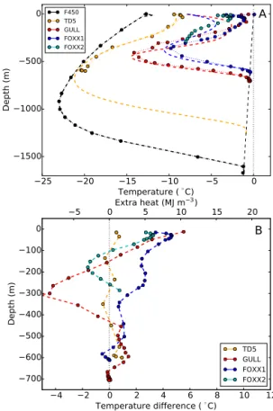
run mD (dissipation only) reveals that measured ice tem-peratures are considerably higher than modeled throughout the ice column (Fig. 5). The maximum extra heat energy of 27 MJ m−3corresponds to a temperature difference of up to 14 K. Following Eq. (1), correcting the temperature differ-ence between the modeled (mD) and observed temperature profiles in the upper part of the model domain would require additional heat from refreezing water equivalent to 9 % by mass.

Adding enhanced dissipation through enhanced shearing ice deformation in the Wisconsin ice (model run mE; Fig. 5) explains the observed extra heat between 500 and 700 m depth. The vertical extent of Wisconsin ice was taken from Ryser et al. (2014b), but the enhancement factor had to be set to 5 instead of the measured (and commonly assumed) value of 3. Since the whole model domain moves at the same ve-locity, the basal ice moves faster than in reality, and therefore has less time to warm. A model run with half surface veloc-ity (not displayed) shows that enough heat is produced at an enhancement factor of 3 to explain measured temperature in the lowest 200 m.

The effect of accumulation of temperate firn (run mF) is shown in Fig. 6. In this model run, the surface temperature between 460–475 km was set to 0◦C, which corresponds to the 160-year time span 1570–1730 C.E. This seemingly arbi-trary horizontal extent of temperate firn conditions coincides with reconstructed warm temperatures at the deep drill sites GRIP and Dye3 (Dahl-Jensen et al., 1998) (see Sect. 4).

4 Discussion

Any shape of temperature profile within the ice can be ob-tained by carefully positioning heat sources during certain time spans within the ice body. The aim of this study is not to perfectly match the observed ice temperature distribution but to investigate how several simple source mechanisms might contribute to the observed temperature profiles. The lower panels of Figs. 5–7 indicate the amount of extra heat per vol-ume needed to match the measured temperatures. This heat is likely provided by several heat sources: dissipation (strain heating), temperate paleo-firn, and cryo-hydrologic warm-ing.

For the ice near the base, strain heating is a crucial process to provide the required 10 MJ m−3of heat (Fig. 5). Calcula-tions with Eq. (2) show that for the considered∼900 years of ice flow the warming is of the order 3 K which is sufficient to explain the measured temperature of the lowest 200 m.

(6)

25 20 15 10 5 0 Temperature (◦C)

1500 1000 500 0

Dep

th

(m)

F450 TD5 GULL FOXX1 FOXX2

0 2 4 6 8 10 12 14 16

Temperature difference (◦C) 700

600 500 400 300 200 100 0

Dep

th

(m)

0 5 10 15 20 25 30

Extra heat (MJ m−3₎

A

B

Figure 5. Measured and modeled temperatures at the three sites Swiss Camp (TD5), GULL and FOXX. Symbols connected by dot-ted lines indicate measurements. Dashed lines refer to the reference model run mD (dissipation only). Solid lines refer to run mE (ad-ditional heat sources from enhanced shear straining in ice-age ice). The scale on top of the lower panel shows the extra heat per volume with respect to model run mD (dissipation only).

temperatures are again warming in the accumulation zone upstream of the study area (Polashenski et al., 2014), and will leave their imprint in the thermal state of the ice sheet. Warm paleo-firn only affects the upper ablation area, and ex-plains only measured temperatures of borehole TD5, but is not sufficient to reproduce warm temperatures at depth at sites GULL and FOXX.

The temperate paleo-firn and ice accumulated in the lower accumulation area is presently emerging as relatively warm ice in the upper ablation area. Further downstream, ice accu-mulated under cold conditions in the dry-snow accumulation area emerges at the surface. Both thermal regimes are clearly visible at our drill sites: at GULL a flat, dirty and slushy ice surface is reminiscent of temperate Alpine glaciers. At FOXX the surface is bright white with many deep cryoconite holes, which is usually found when cold ice emerges in the ablation area (e.g., Ryser et al., 2013). Our near-surface tem-perature profiles (Fig. 2a) support this notion, with temper-atures above −2◦C at GULL, but colder near-surface tem-peratures at downstream drill site FOXX. It is likely this dif-ference in surface temperature, and therefore the distribution

25 20 15 10 5 0

Temperature (◦C) 1500

1000 500 0

Dep

th

(m)

0 2 4 6 8 10 12 14 16

600 500 400 300 200 100 0

Dep

th

(m)

0 5 10 15 20 25 30

A

B

Figure 6.Same as Fig. 5 but for model run mEF (enhanced shear straining and temperate paleo-firn).

of dust (dirty ice vs. cryoconite holes) that leads to the dark band visible in the upper ablation zone of the western GrIS (Wientjes and Oerlemans, 2010; Wientjes et al., 2012).

For the central ice body an important heat source is needed to provide the 25 MJ m−3 heat, corresponding to the ob-served 12–14 K temperature difference at GULL and FOXX (Fig. 5). Strain heating due to horizontal stress gradients is one possible heat source. Caterpillar-like horizontal ex-tension and compression on diurnal and longer time scales has been observed in the study area (Ryser et al., 2014a). This heat source is, however, not strong enough: a quick calculation with Eq. (2), A (−10◦C) and a continuous, very high horizontal–longitudinal stress gradient of 0.1 MPa yields a heat production of only 0.0011 MJ m−3a−1which is one order of magnitude lower than the shear strain-induced heating of basal ice discussed above.

(7)

25 20 15 10 5 0 Temperature (◦C)

1500 1000 500 0

Dep

th

(m)

4 2 0 2 4 6 8 10 12

600 500 400 300 200 100 0

Dep

th

(m)

5 0 5 10 15 20

A

B

Figure 7.Same as Fig. 5 but for model run mCEF (crevasses, en-hanced shear straining, and temperate paleo-firn).

to the drill site, its depth would have to be of the order of 400 m, and it would need to provide a temperature of 0◦C for 100 years. Figure 7 shows results from a model run assum-ing a series of crevasses of 400 m depth and 100 m spacassum-ing which provide a temperature of 0◦C for 50 years.

Very deep crevasses (300–400 m) with tens of years of ac-tivity are only possible if they are water-filled (Van der Veen, 1998), but do not penetrate to the bottom. While there is hy-drofracturing as a mechanism to create a deep crevasse, there must be a mechanism to stop their depth penetration. Limited water supply for hydrofracturing is one possible cause, which is very likely within the small upstream surface area within a crevasse field. Another possible limiting factor for crevasse penetration to the bed is tougher ice at the bottom. The criti-cal crack-tip loading rate at −20◦C is orders of magnitude lower than at temperatures approaching the melting point (Schulson and Duval, 2009, Table 9.1). We therefore sug-gest that water-driven crevasses stop their downwards growth once they reach warmer ice. If such very deep, water-filled crevasses indeed exist is unknown, although some observa-tional evidence of strong englacial reflectors was detected in the study area (Catania et al., 2008; Catania and Neumann, 2010). These strong reflectors are likely due to water stored within the glacier ice.

An alternative explanation to crevasses are moulins, ver-tical shaft systems draining water from the surface. Moulins are stationary drainage features on an undulating surface, and are only active for a few years until they move out of sur-face depressions (Catania and Neumann, 2010). Their spac-ing along a flow line amounts to the duration of their activity times the flow velocity, and thus hundreds of meters in the area of our drill sites (Thomsen et al., 1988; Phillips et al., 2011). A series of model runs was performed that implement moulins as vertical shafts at melting temperature during their activity (Vorkauf, 2014). As line sources they provide little warming to the surrounding ice. Modeled temperature differ-ence at the site of a moulin is below 1 K after 10 years of in-activity (Vorkauf, 2014). Furthermore, modeled vertical pat-terns of ice temperature around moulins do not agree with the observed temperature profiles. Therefore we conclude that very deep water-filled crevasses, rather than moulins, are the main heat sources in the ablation area.

An earlier modeling study of thermal properties in the same area (Phillips et al., 2013) concluded that ice warmed by cryo-hydrologic features has an important influence on ice deformation rates, and is causing the increasing flow veloci-ties observed at the surface. The main difference in modeling approaches is their assumption of continuous heat sources spread over the entire ice thickness. Neither our data nor the interpretation with the heat flow model support this assump-tion. The ice in the lowest 200 m of the ice column shows no signs of warming through cryo-hydrologic features, as the temperatures there can be explained by diffusion and dissipa-tion alone, as shown in Fig. 5. Since vertical shear deforma-tion is highest at depth (Ryser et al., 2014a, b), temperature changes in the central ice body will have a minor influence on ice deformation rates, and therefore surface velocities.

A noteworthy feature of the presented ice temperature pro-files is the difference between the two propro-files at site FOXX (Fig. 2). The temperature difference between the two bore-holes which are 86 m apart amounts to 4 K in 200–300 m depth. Furthermore, the profiles intersect below 300 m depth. Only a combination of very localized heat sources can pro-duce these different shapes of the temperature profiles in such close vicinity. No simple heat source patterns, nor the influ-ence of active vertical moulins or horizontal conduits pro-duce similar temperature profiles (Vorkauf, 2014). The obser-vation of very different temperature patterns in neighboring boreholes cautions against interpretation of single boreholes in areas where englacial heat sources strongly affect the ther-mal structure of the ice.

5 Conclusions

(8)

study: dissipation, temperate paleo-firn, and cryo-hydrologic features, represented by very deep water-filled crevasses.

An important conclusion of the modeling study is that tem-perate firn was accumulated in the now cold accumulation area during a warm period of about 160 years, during 1570– 1730 C.E. (Dahl-Jensen et al., 1998). This temperate paleo-firn is presently emerging as relatively warm ice in the upper ablation area, and is likely the cause for the observed dark band in the ablation area of the western GrIS (Wientjes and Oerlemans, 2010; Wientjes et al., 2012).

Future warming of the firn areas of the GrIS by extreme melt events, such as in summer 2012 (McGrath et al., 2013), are likely in a warming Arctic. Extended areas of surface melt might lead to increasing firn temperatures, affecting large parts of the ice sheet. Such recent warming has already been detected in the study area (Polashenski et al., 2014).

The central ice body at our study sites is 10–15 K warmer than modeled with heat diffusion alone. To heat this ice to observed temperatures, a continuous heat source with melt-ing point temperature is required which penetrates down to 300–400 m below the surface. The most likely sources are very deep, water-filled crevasses which persist for decades as they move through the extensional stress regime of a crevasse zone.

All of these heat sources were inferred from compari-son of models with measurements. How important localized sources, such as crevasses and moulins, are for the thermal regime of the ice is still a matter of debate. Sampling ice tem-perature at sites suited for drilling (un-crevassed depressions with surface streams) yields a skewed picture of the full vari-ability encountered in nature. Without a systematic sampling of ice temperatures to great depth, the information content extracted from individual holes is to be taken with care. This argument is impressively illustrated by the two temperature profiles from site FOXX which are 86 m apart, but show large differences in the upper 300 m, and even cross below.

Acknowledgements. We thank several people who were essential

in this project: Cornelius Senn, Edi Imhof, Thomas Wyder, An-dreas Bauder, Christian Birchler, Michael Meier, Blaine Moriss, and Fabian Walter. We acknowledge the constructive reviews by Martin Truffer and two anonymous referees.

This project was supported by Swiss National Science Foun-dation Grant 200021_127197, US-NSF Grants OPP 0908156, OPP 0909454 and ANT-0424589 (to CReSIS), NASA Cryospheric Sciences, and Climate Modeling Programs within the US Depart-ment of Energy Office of Science. Logistical support was provided by CH2MHill Polar Services.

Edited by: I. M. Howat

References

Ahlstrom, A. P.: Previous glaciological activities related to hy-dropower at Paakitsoq, Ilulissat, West Greenland, Tech. Rep., 25, Danmarks og Grønlands Geologiske Undersøgelse, 2007. Andrews, L. C., Catania, G. A., Hoffman, M. J.,

Gul-ley, J. D., Lüthi, M. P., Ryser, C., HawGul-ley, R. L., and Neumann, T. A.: Direct observations of evolving subglacial drainage beneath the Greenland Ice Sheet, Nature, 514, 80–83, doi:10.1038/nature13796, 2014.

Box, J. E.: Greenland Ice Sheet mass balance reconstruction, Part II: Surface mass balance (1840–2010), J. Climate, 26, 6974–6989, doi:10.1175/JCLI-D-12-00518.1, 2013

Budd, W., Jacka, T., Jenssen, D., Radok, U., and Young, N.: Derived physical characteristics of the Greenland Ice Sheet, Meteor. Dept. Pub. no. 23, University of Melbourne, Melbourne, 1982. Catania, G. A. and Neumann, T. A.: Persistent englacial drainage

features in the Greenland Ice Sheet, Geophys. Res. Lett., 37, L02501, doi:10.1029/2009GL041108, 2010.

Catania, G. A., Neumann, T. A., and Price, S. F.: Characterizing englacial drainage in the ablation zone of the Greenland ice sheet, J. Glaciol., 54, 567–578, doi:10.3189/002214308786570854, 2008.

Cuffey, K. and Paterson, W.: The Physics of Glaciers, Elsevier, Burlington, MA, USA, 2010.

Dahl-Jensen, D., Mosegaard, K., Gundestrup, N., Clow, G. D., Johnsen, S. J., Hansen, A. W., and Balling, N.: Past temperatures directly from the Greenland Ice Sheet, Science, 282, 268–271, doi:10.1126/science.282.5387.268, 1998.

DTU Space, M. and Remote Sensing, Lyngby, D.: Ice radar data, unpublished data, 2005.

Forster, R. R., Box, J. E., van den Broeke, M. R., Mièège, C., Burgess, E. W., van Angelen, J. H., Lenaerts, J. T. M., Koenig, L. S., Paden, J., Lewis, C., Gogineni, S. P., Leuschen, C., and McConnell, J. R.: Extensive liquid meltwater storage in firn within the Greenland ice sheet, Nat. Geosci., 7, 418–422, doi:10.1038/NGEO2043, 2013.

Funk, M., Echelmeyer, K., and Iken, A.: Mechanisms of fast flow in Jakobshavns Isbrae, Greenland; Part II: Modeling of englacial temperatures, J. Glaciol., 40, 569–585, 1994.

Gogineni, P.: CReSIS Greenland Radar Data, Lawrence, Kansas, USA, Digital Media, available at: http://data.cresis.ku.edu/ (last access: 1 October 2013), 2012.

Greve, R.: Application of a polythermal three-dimensional ice sheet model to the Greenland ice sheet: response to a steady-state and transient climate scenarios, J. Climate, 10, 901–918, 1997. Harper, J., Humphrey, N., Pfeffer, W., Brown, J., and

Fet-tweis, X.: Greenland ice-sheet contribution to sea-level rise buffered by meltwater storage in firn, Nature, 491, 240–243, doi:10.1038/nature11566, 2012.

Humphrey, N. F., Harper, J. T., and Pfeffer, W. T.: Thermal track-ing of meltwater retention in Greenland’s accumulation area, J. Geophys. Res., 117, F01010, doi:10.1029/2011JF002083, 2012. Hutter, K. and Jöhnk, K.: Continuum Methods of Physical Model-ing: Continuum Mechanics, Dimensional Analysis, Turbulence, Springer, Berlin, Germany, 2004.

(9)

Joughin, I., Das, S. B., King, M. A., Smith, B. E., Howat, I. M., and Moon, T.: Seasonal speedup along the western flank of the Greenland Ice Sheet, Science, 320, 781–783, 2008.

Kirk, B., Peterson, J. W., Stogner, R. H., and Carey, G. F.: libMesh: a C++ library for parallel adaptive mesh re-finement/coarsening simulations, Eng. Comput., 22, 237–254, doi:10.1007/s00366-006-0049-3, 2006.

Letreguilly, A., Reeh, N., and Huybrechts, P.: The Greenland ice sheet through the last glacial-interglacial cycle, Palaeogeogr. Palaeocl., 90, 385–394, 1991.

Lüthi, M. P., Funk, M., Iken, A., Gogineni, S., and Truf-fer, M.: Mechanisms of fast flow in Jakobshavns Isbrae, Green-land; Part III: Measurements of ice deformation, temperature and cross-borehole conductivity in boreholes to the bedrock, J. Glaciol., 48, 369–385, doi:10.3189/172756502781831322, 2002.

McGrath, D., Colgan, W., Bayou, N., and Steffen, K.: Recent warm-ing at Summit, Greenland: global context and implications, Geo-phys. Res. Lett., 40, 2091–2096, doi:10.1002/grl.50456, 2013. Phillips, T., Rajaram, H., and Steffen, K.: Cryo-hydrologic

warm-ing: a potential mechanism for the thermal response of ice sheets, Geophys. Res. Lett., 37, L20503, doi:10.1029/2010GL044397, 2010.

Phillips, T., Leyk, S., Rajaram, H., Colgan, W., Abdalati, W., Mc-Grath, D., and Steffen, K.: Modeling moulin distribution on Ser-meq Avannarleq glacier using ASTER and WorldView imagery and fuzzy set theory, Remote Sens. Environ., 115, 2292–2301, doi:10.1016/j.rse.2011.04.029, 2011.

Phillips, T., Rajaram, H., Colgan, W., Steffen, K., and Abdalati, W.: Evaluation of cryo-hydrologic warming as an explanation for increased ice velocities in the wet snow zone, Sermeq Avan-narleq, West Greenland, J. Geophys. Res.-Earth, 118, 1241– 1256, doi:10.1002/jgrf.20079, 2013.

Polashenski, C., Courville, Z., Benson, C., Wagner, A., Chen, J., Wong, G., Hawley, R., and Hall, D.: Observations of pro-nounced Greenland ice sheet firn warming and implications for runoff production, Geophys. Res. Lett., 41, 4238–4246, doi:10.1002/2014GL059806, 2014.

Ryser, C., Lüthi, M., Blindow, N., Suckro, S., Funk, M., and Bauder, A.: Cold ice in the ablation zone: its relation to glacier hydrology and ice water content, J. Geophys. Res., 118, 693– 705, doi:10.1029/2012JF002526, 2013.

Ryser, C., Lüthi, M. P., Andrews, L. C., Hoffman, M. J., Catania, G. A., Hawley, R. L., and Neumann, T. A.: Caterpillar-like ice motion in the ablation zone of the Greenland Ice Sheet, J. Geo-phys. Res.-Earth, 119, 2258–2271, doi:10.1002/2013JF003067, 2014a.

Ryser, C., Lüthi, M., Andrews, L., Hoffman, M., Catania, G., Haw-ley, R., Neumann, T., and Kristensen, S. S.: Sustained high basal motion of the Greenland Ice Sheet revealed by borehole defor-mation, J. Glaciol., 60, 647–660, doi:10.3189/2014JoG13J196, 2014b.

Schulson, E. and Duval, P.: Creep and Fracture of Ice, Cambridge University Press, 2009.

Thomsen, H. H. and Thorning, L.: Ice Temperature Profiles for Western Greenland, Tech. rep., Groenl. Geol. Unders., Copen-hagen, 1992.

Thomsen, H. H., Thorning, L., and Braithwaite, R. J.: Glacier-Hydrological conditions on the inland ice North-East of Jakob-shavn/Ilusissat, West Greenland, Report 138, Grønlands Geolo-giske Undersøgelse, Copenhagen, Denmark, 1988.

Thomsen, H. H., Olesen, O., Braithwaite, R. J., and Boggild, C.: Ice drilling and mass balance at Pakitsoq, Jakobshavn, central West Greenland, Report 152, Grønlands Geologiske Undersøgelse, Copenhagen, Denmark, 1991.

Van der Veen, C. J.: Fracture mechanics approach to penetration of surface crevasses on glaciers, Cold Reg. Sci. Technol., 27, 31–47, 1998.

Vorkauf, M.: Modeling the influence of moulins and temperate firn on the vertical temperature profile of the Greenland Ice Sheet, Master’s thesis, VAW, ETH Zürich, Switzerland, 2014.

Wientjes, I. G. M. and Oerlemans, J.: An explanation for the dark region in the western melt zone of the Greenland ice sheet , The Cryosphere, 4, 261–268, doi:10.5194/tc-4-261-2010, 2010. Wientjes, I., van de Wal, R., Schwikowski, M., Zapf, A., Fahrni,