Impact of HONO on global atmospheric chemistry calculated with an empirical parameterization in the EMAC model

(1)

ACPD

12, 12885–12934, 2012

Impact of HONO on global atmospheric

chemistry

Y. F. Elshorbany et al.

Title Page

Abstract Introduction

Conclusions References

Tables Figures

◭ ◮

Back Close

Full Screen / Esc

Printer-friendly Version Interactive Discussion

Discussion

P

a

per

|

Dis

cussion

P

a

per

|

Discussion

P

a

per

|

Discussio

n

P

a

per

|

Atmos. Chem. Phys. Discuss., 12, 12885–12934, 2012 www.atmos-chem-phys-discuss.net/12/12885/2012/ doi:10.5194/acpd-12-12885-2012

Atmospheric Chemistry and Physics Discussions

This discussion paper is/has been under review for the journal Atmospheric Chemistry and Physics (ACP). Please refer to the corresponding final paper in ACP if available.

Impact of HONO on global atmospheric

chemistry calculated with an empirical

parameterization in the EMAC model

Y. F. Elshorbany1, B. Steil1, C. Br ¨uhl1, and J. Lelieveld1,2

1

Max-Plank Institute for Chemistry, Atmospheric Chemistry Department, Mainz, Germany 2

The Cyprus Institute, Nicosia, Cyprus, and King Saud University, Riyadh, Saudi Arabia

Received: 23 April 2012 – Accepted: 10 May 2012 – Published: 23 May 2012

Correspondence to: Y. F. Elshorbany (yasin.elshorbany@mpic.de)

Published by Copernicus Publications on behalf of the European Geosciences Union.

(2)

ACPD

12, 12885–12934, 2012

chemistry

Title Page

Tables Figures

◭ ◮

Back Close

Full Screen / Esc

Discussion

P

a

per

|

Dis

cussion

P

a

per

|

Discussion

P

a

per

|

Discussio

n

P

a

per

|

Abstract

The photolysis of HONO is important for the atmospheric HOx(OH+HO2) radical

bud-get and ozone formation, especially in polluted air. Nevertheless, owing to the incom-plete knowledge of HONO sources, realistic HONO mechanisms have not yet been implemented in global models. We investigated measurement data sets from 15 field

5

measurement campaigns conducted in different countries worldwide. It appears that the HONO/NO_x ratio is a good proxy predictor for HONO mixing ratios under diff er-ent atmospheric conditions. From the robust relationship between HONO and NOx,

a representative mean HONO/NOx ratio of 0.02 has been derived. Using a global

chemistry-climate model and employing this HONO/NO_x ratio, realistic HONO levels

10

are simulated, being about one order of magnitude higher than the reference calcula-tions, which only consider the reaction OH+NO→HONO. The resulting enhancement of HONO significantly impacts HOxlevels and photo-oxidation products (e.g, O3, PAN),

mainly in polluted regions. Furthermore, the relative enhancements in OH and sec-ondary products were higher in winter than in summer, thus enhancing the oxidation

15

capacity in polluted regions, especially in winter, when the other photolytic OH sources are of minor importance. Our results underscore the need to improve the understanding of HONO chemistry and its representation in atmospheric models.

1 Introduction

Since three decades, nitrous acid (HONO) photolysis has been shown to be an

impor-20

tant source of OH radicals, especially during the early morning, when other sources are of minor importance (Perner and Platt, 1979; Harris et al., 1982). Recently, HONO pho-tolysis was reported to contribute more strongly to daytime primary OH production than O3photolysis, both under urban and rural conditions (Elshorbany et al., 2009a; S ¨orgel

et al., 2011a, respectively). It has been demonstrated that HONO photolysis can be

25

(3)

ACPD

12, 12885–12934, 2012

chemistry

Title Page

Tables Figures

◭ ◮

Back Close

Full Screen / Esc

Discussion

P

a

per

|

Dis

cussion

P

a

per

|

Discussion

P

a

per

|

Discussio

n

P

a

per

|

et al., 2009a, 2010a; Ren et al., 2006; Dusanter et al, 2009) as well as low NO_x con-ditions (e.g., Kleffmann et al., 2005; Elshorbany et al., 2012, S ¨orgel et al., 2011a). OH radicals constitute the major oxidant of the atmosphere, initiating the removal of most reactive gases (i.e. regulating the self-cleaning capacity of the atmosphere), though also lead to the formation of secondary products such as O3 and PAN, which can be 5

harmful for human health. The OH oxidation of volatile organic compound (VOC) con-tributes to the formation of aerosol particles, affecting air quality and climate. HONO is also an important ingredient of the strongly anthropogenically perturbed global nitrogen cycle, which indirectly influences climate change (Kumala and Pet ¨aj ¨a, 2011).

Owing to the thus far incomplete knowledge of HONO sources, in particular during

10

daytime, it was not yet possible to simulate realistic HONO levels using global models. Li et al. (2010), Zhang et al. (2011) and Czader et al. (2012) have shown that additional HONO sources are required to match measured HONO mixing ratios; for some regions tenfold mismatches have been found based on the known gas phase HONO formation only (i.e., OH+NO→HONO). Li et al. (2011) and Goncalves et al. (2012) showed that

15

modelled HONO was consistently lower than observations, even when the most eff ec-tive recently suggested formation mechanisms were considered. This underestimation of HONO by models may be expected to impact the simulated HOxand O3budgets as

well as other secondary products.

Several HONO sources have been identified in the laboratory (e.g., Zhou et al.,

20

2003; George et al., 2005; Stemmler et al., 2006, 2007; Bejan et al., 2006; Li et al., 2008; Gustafsson et al., 2006; Ndour et al., 2008; Su et al., 2011), yet these sources cannot account for the HONO levels observed during daytime (Elshorbany et al., 2010b; Su et al., 2011; Czader et al., 2012). While the heterogeneous conversion of NO2 on humid surfaces (Finlayson-Pitts et al., 2003) in the dark is commonly ac-25

cepted as the dominant HONO source during the night (Alicke et al., 2002), the exact mechanism is still unclear. For daytime HONO sources, five photochemical mecha-nisms were recently identified. Three of them dominate under high-NOx urban

condi-tions, i.e., heterogeneous conversion of gaseous NO₂on photosensitized solid surface

(4)

ACPD

12, 12885–12934, 2012

chemistry

Title Page

Tables Figures

◭ ◮

Back Close

Full Screen / Esc

Discussion

P

a

per

|

Dis

cussion

P

a

per

|

Discussion

P

a

per

|

Discussio

n

P

a

per

|

organic compounds (George et al., 2005; Stemmler et al., 2006), photocatalytic con-version of NO2on TiO2(Gustafsson et al., 2006; Ndour et al., 2008) and the photolysis

of gaseous nitro-aromatic compounds (Bejan et al., 2006), which are expected to cor-relate well with j(NO₂). Under low-NO_x rural conditions, the photolysis of nitric acid (Zhou et al., 2003, 2011) adsorbed on solid surfaces (including vegetation) may

domi-5

nate and is expected to primarily correlate withj(O1D), related to the much lower wave-length range of nitric acid photolysis thanj(NO₂). Su et al. (2011) showed that HONO can also be emitted from soils, being a function of temperature (i.e, light independent). This source may be important in tropical forested regions. S ¨orgel et al. (2011a) showed that unknown HONO daytime sources, normalized with NO₂mixing ratios have a clear

10

dependency onj(NO₂). Recently, Czader et al. (2012) also showed that photo-induced conversion of NO2on organic surfaces is a strong daytime HONO source.

In addition to the incomplete knowledge about daytime HONO chemistry, most of the thus far identified HONO sources are generally also associated with large uncertainty as the mechanisms and controlling parameters are only partly understood (Kleffmann,

15

2007; Li et al., 2010; Czader et al., 2012; Goncalves et al., 2012). Consequently, sev-eral recent attempts to simulate HONO formation were based on the modulation of the model parameters (i.e., via several assumptions and simplifications) to match the mea-surements in individual studies (e.g., Li et al., 2010; Czader et al., 2012; Goncalves et al., 2012). For example, Czader et al. (2012) simulated HONO using an approach

20

adopted by Li et al. (2010), for which a daytime HONO source with a relatively large uptake coefficient was employed based on variable threshold values of light intensity. However, Czader et al. (2012) obtained unrealistically high HONO concentrations and therefore used the same uptake coefficient but scaled by a different and constant fac-tor to match the measured HONO. In contrast, Goncalves et al. (2012) obtained about

25

(5)

ACPD

12, 12885–12934, 2012

chemistry

Title Page

Tables Figures

◭ ◮

Back Close

Full Screen / Esc

Discussion

P

a

per

|

Dis

cussion

P

a

per

|

Discussion

P

a

per

|

Discussio

n

P

a

per

|

in global models, as each region would need its specific parameterization. Thus, a more general approach is needed to calculate more realistic HONO levels on a global scale. A common factor between the known major day- and nighttime sources is that they are generally surface-based (except the gas phase photolysis of nitro-aromatic com-pounds). Indeed, such HONO sources contribute a major fraction of measured HONO

5

levels (Harrison and Kitto, 1994; Stutz et al., 2002; Veitel, 2002; Kleffmann et al., 2003; Zhang et al., 2009; S ¨orgel et al., 2011b; Wong et al., 2011) and consequently the dis-persion into the atmosphere is a function of turbulent mixing (S ¨orgel et al. 2011b). This was first proposed by Febo et al. (1996) based on radon measurements, a species emitted exclusively from the ground. Veitel (2002) also showed that HONO correlates

10

linearly with radon with highest values reported in winter. In addition, both, ground-and aircraft-based gradient measurements showed that HONO mixing ratios near to the ground follow a steep gradient during stable conditions (Veitel, 2002; Zhang et al., 2009, respectively). Thus, HONO mixing ratios appear to be controlled by the sur-face area in a mixed volume of air (s/v), and the changes can often be accounted

15

for by scaling HONO to NO2 or NOx (S ¨orgel et al. 2011b, and references therein).

Similarly, Zhang et al. (2011) showed that the spatial distribution of simulated HONO during day- and nighttime is generally consistent with the NOx emission pattern. Kleff

-mann (2007) concluded that the HONO/NOx ratio is a reasonable measure of HONO

as it takes into account the dilution of trace gases during transport, after being emitted

20

or formed at the ground. Several previous studies indicated the HONO/NOx ratio as

a proxy for HONO formation under rural (e.g., Acker et al., 2006; Elshorbany et al., 2012; S ¨orgel et al., 2011b), remote (e.g., Kleffmann and Wiesen, 2008) and urban conditions (e.g., Elshorbany et al., 2009a, 2010a). Furthermore, Villena et al. (2011) showed that the HONO/NOx ratio and its daytime maximum are independent of alti-25

tude. Thus, the HONO/NO_xratio may be a practicable metric to help predict HONO in the atmosphere.

In this study, data sets from 15 different field measurement campaigns around the globe are investigated, confirming that the HONO/NO_xratio is a good proxy predictor of

(6)

ACPD

12, 12885–12934, 2012

chemistry

Title Page

Tables Figures

◭ ◮

Back Close

Full Screen / Esc

Discussion

P

a

per

|

Dis

cussion

P

a

per

|

Discussion

P

a

per

|

Discussio

n

P

a

per

|

the HONO mixing ratio for use in global models. The impacts of simulated HONO levels on the levels of oxidants (OH, O3, PAN, etc.) are determined using an atmospheric

chemistry-climate model.

2 Methodology

2.1 Model description

5

The applied modelling system is based on the ECHAM5 general circulation model (Roeckner et al., 2006) and the Modular Earth Submodel System (MESSy, J ¨ockel et al., 2005) to simulate the meteorology and atmospheric chemistry. The ECHAM5/MESSy Atmospheric Chemistry (EMAC) system is a coupled lower-middle atmospheric chem-istry general circulation model (AC-GCM), which has been extensively evaluated (e.g.,

10

J öckel et al., 2006; Lelieveld et al., 2007; Tost et al., 2007; Pozzer et al., 2008, 2010, 2012; Br ühl et al., 2012). The model structure and setup have been described by J öckel et al. (2006) and only a brief description is given here.

Atmospheric chemical reactions are incorporated in the model through the module MECCA1 (Sander et al., 2005), including the Mainz Isoprene Mechanism, version 2

15

(MIM2, P ¨oschl et al., 2000; von Kuhlmann et al., 2004; Taraborrelli et al., 2009). To study the effects of changes in the chemistry while avoiding possible feedbacks of ra-diatively active gases and aerosols through the meteorology, the radiation scheme has been decoupled, and the model is used in the atmospheric chemistry-transport mode. The radiation code in EMAC therefore uses an ozone climatology (Fortuin and Kelder,

20

1998), fixed vertical profiles for CH₄, N₂O and CFCs and constant mixing ratios of CO₂. The reference run (base) has been performed for the year 2005 in T42L31 resolution (i.e., with a triangular truncation at wave number 42 for the spectral core of ECHAM5, and with 31 levels on a hybrid-pressure grid in the vertical, reaching up to 10 hPa). The T42 resolution corresponds to a quadratic Gaussian grid of approximately 2.8◦×2.8◦ 25

(7)

ACPD

12, 12885–12934, 2012

chemistry

Title Page

Tables Figures

◭ ◮

Back Close

Full Screen / Esc

Discussion

P

a

per

|

Dis

cussion

P

a

per

|

Discussion

P

a

per

|

Discussio

n

P

a

per

|

“nudging” towards actual meteorology by the assimilation of analysis data from the European Centre for Medium-range Weather Forecasting (ECMWF) through the New-tonian relaxation of four prognostic model variables: temperature, divergence, vorticity and the logarithm of surface pressure (van Aalst et al., 2004). The first 5 months of the simulation are regarded as spin up period and these results are not considered in our

5

analysis.

Output has been archived as 1-hourly instantaneous fields to capture an hourly re-solved diurnal cycle. In the sensitivity runs S1, S2 and S3, HONO levels were parame-terized such that the HONO/NOxratio is fixed at 0.01, 0.02 and 0.04, respectively (see

Sect. 3.3). This was achieved by an iterative correction of HONO and NOx(i.e., without 10

disturbing the reactive nitrogen budget), which was applied every minute, thus limiting deviations in the HONO/NOxratio to within±0.005.

2.2 Field measurements

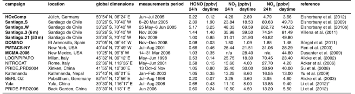
Average diurnally resolved data sets from eight different field measurement campaigns (see Table 1) were used to analyse the day- and nighttime HONO chemistry.

HOx-15

Comp took place at the J ¨ulich Research Centre, Germany during 9–11 July, 2005 (we used only the diurnal profile of the cloud free day, 10 July, Elshorbany et al., 2012); the Santiago de Chile campaigns took place during 8–20 March 2005 (Santiago S, Elshorbany et al., 2009a) and during 25 May to 7 June 2005 (Santiago W, diurnal av-erage of cloud free days only, Elshorbany et al., 2010a); the PMTACS-NY campaign

20

took place from 10 July to 2 August 2001 in New York (New York, Ren et al., 2003); the Mexico City Metropolitan Area campaign took place during 14–31 March 2006 (MCMA-2006, Dusanter et al., 2009); the DOMINO campaign took place in Southwest-ern Spain during November–December, 2008 (DOMINO, diurnal average of cloud free days only, S ¨orgel et al., 2011a) and we used two gradient measurement data sets

ob-25

tained during a field measurement campaign at a 55 m tall building in Santiago de Chile from 17–29 November 2009 at the altitudes of 6 m (3rd floor, Santiago 3) and 53 m (21st floor, Santiago 21) above the ground (Villena et al., 2011). In addition, measured

(8)

ACPD

12, 12885–12934, 2012

chemistry

Title Page

Tables Figures

◭ ◮

Back Close

Full Screen / Esc

Discussion

P

a

per

|

Dis

cussion

P

a

per

|

Discussion

P

a

per

|

Discussio

n

P

a

per

|

average concentrations of HONO and NO_xfrom 7 other field measurement campaigns, adopted from Li et al. (2012), were also investigated (see Table 1). These measurement campaigns were performed in three different continents (from 52◦N to 37◦S and from 116◦E to 99◦W) under a range of meteorological conditions. These measurements also encompass a wide range of different NOx conditions, typically from NO sensi-5

tive conditions (e.g., HOxComp) to VOC sensitive conditions (e.g., Santiago and New York). Furthermore , the results obtained from the analysis of these data are compared with other field campaigns reported in the literature. The range of HONO mixing ratios obtained from these data sets represents the minimum and maximum HONO levels measured during the last decade and therefore, represent an optimal global overview

10

of HONO measurements.

2.3 Intercomparison of field measurements

The average measured diurnal profiles of HONO, HONO/NOx and j(NO2) for the first

8 data sets in Table 1 are shown in Figs. 1 and 2. The HONO diurnal profiles typically show increasing mixing ratios after sunset due to HONO formation by heterogeneous

15

reactions, direct emissions and the absence of photolytic loss processes, in addition to the decrease in boundary layer height (i.e. the mixing volume). Owing to its short lifetime of about 10–30 min and the increased vertical mixing, HONO decreases after sunrise, reaching its minimum levels during the afternoon. Influenced by relatively high nighttime values, 24 h average HONO levels range from about 0.1 to 5 ppbv (see Table

20

1). Average daytime HONO mixing ratio range from about 3.25 ppbv in Santiago de Chile (winter) to about 0.03 ppbv during the DOMINO campaign in Southern Spain (autumn). Daytime HONO/NOx ratios range from about 0.01 during the MCMA-2006

to about 0.05 during the Santiago S with average and median values of about 0.02 for all campaigns. The very low values of the HONO/NOx ratio during MCMA-2006 in 25

(9)

ACPD

12, 12885–12934, 2012

chemistry

Title Page

Tables Figures

◭ ◮

Back Close

Full Screen / Esc

Discussion

P

a

per

|

Dis

cussion

P

a

per

|

Discussion

P

a

per

|

Discussio

n

P

a

per

|

Average diurnal profiles of gradient HONO measurements in Santiago de Chile at 6 and 53 m altitude are shown in Fig. 2. The diurnal profiles show a clear vertical gradient with HONO mixing ratios at 53 m of about 60 % of those at 6 m during daytime. Similar HONO gradient were observed previously in the Mexico City metropolitan area during the MCMA-2003 at 70 and 16 m altitude (Volkamer et al., 2010). Both NO and NO2 5

show similar gradients while O3 increases with height owing to the inter-conversion of

NO/NO₂through reactions of NO (emitted at ground level) with RO₂ and HO₂ (Villena et al., 2011). Due to the stronger absolute gradient of NO2, HONO/NO2 ratios show

an opposite strong gradient during daytime while HONO/NOx ratios appear to be

al-most unaffected. Similarly, Kleffmann (2007) also showed that the HONO/NO_x ratio

10

decreases only little with altitude from about 2.5 % at 10 m to about 2 % at 190 m. The photolysis of HONO releasing OH and NO, enhances photochemical oxidation pro-cesses, which subsequently catalytically convert NO into NO2which in turn photolyses

to form O₃. Consequently, the relative change of HONO as a result of its photolysis is also reflected in the O3 and NOx levels resulting in a nearly constant HONO/NOx 15

ratio. Therefore, the HONO/NO2 ratio may be considered a good measure of HONO

during the night (see also S ¨orgel et al., 2011b) while during daytime the HONO/NO_x ratio seems to be more suited (see Sect. 3.3).

3 Results and discussion

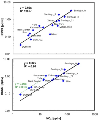
3.1 Average HONO/NOxratio

20

To obtain an overview of measured HONO/NO_x ratios, daytime and 24 h average mix-ing ratios of HONO and NOx based on all available data sets are plotted in Fig. 3.

A high correlation (R2=0.87) is obtained between HONO and NOxduring daytime with

a linear regression slope of 0.02±0.002 (Fig. 3, upper panel). Similarly, a high corre-lation (R2=0.90) is obtained for the 24 h average values with a linear regression slope

25

(10)

ACPD

12, 12885–12934, 2012

chemistry

Title Page

Tables Figures

◭ ◮

Back Close

Full Screen / Esc

Discussion

P

a

per

|

Dis

cussion

P

a

per

|

Discussion

P

a

per

|

Discussio

n

P

a

per

|

(Back Garden), Yufa and Kathmandu campaigns, a slightly different regression slope of 0.05 (±0.004) was found (Fig. 3, lower panel). This is likely due to the relatively high NO2/NOx ratio during these campaigns (see Table 1), especially during night when

the influence of direct NO emissions in these regions is small. These measurement campaigns were characterised by a high NO morning peak, decreasing to less than

5

1 ppbv during the rest of the day due to a change in wind direction as mentioned in the respective references (S ¨orgel et al., 2011a; Alicke et al., 2003; Elshorbany et al., 2012; Li et al., 2012; Yu et al., 2009, respectively, except for the Yufa campaign, for which the data were obtained from Li et al. (2012)). The higher NO2 fraction during

the night leads to higher HONO via its heterogeneous formation in the dark, resulting

10

in higher HONO/NO_x ratios compared to other measurement campaigns. This influ-ence is less pronounced during daytime as the NO2/NOx ratios for all campaigns are

much closer (see Table 1). Since HONO photolysis only influences HOx, O3and other

oxidants during daytime, the HONO/NO_xregression slope of 0.02±0.001 determined

above appears to be representative and may be used to investigate the impact on HOx 15

and oxidant chemistry. Detailed analyses of the factors controlling the HONO diurnal profile as a function of NO_xare presented in the next section.

3.2 HONO diurnal profile

To determine the factors controlling the HONO mixing ratio as a function of NOx, the

aforementioned 8 field measurement data sets (HOxComp, Santiago S, Santiago W,

20

Santiago 3, Santiago 21, DOMINO, MCMA-2006 and New York) have been investi-gated. During the first 6 measurement campaigns, HONO was measured by the sensi-tive LOPAP (Long Path Absorption Photometer) technique (Heland et al., 2001; Kleff -mann et al., 2002). During MCMA-2006, HONO was measured using LP-DOAS (Du-santer et al., 2009 and references therein), while during the New York campaign HONO

25

(11)

ACPD

12, 12885–12934, 2012

chemistry

Title Page

Tables Figures

◭ ◮

Back Close

Full Screen / Esc

Discussion

P

a

per

|

Dis

cussion

P

a

per

|

Discussion

P

a

per

|

Discussio

n

P

a

per

|

B), mid-noon to sunset (sector C) and from sunset to midnight (sector D), grouped into two main sectors, nighttime (A and D) and daytime (B and C). The onset of sunrise and sunset is defined at 30 % of the maximum measuredj(NO2) values. The duration

of each sector period varies based on thej(NO₂) values measured in each study. The obtained linear regression expression is then used to calculate HONO mixing ratios in

5

each sector in terms of NOxand the other related parameters.

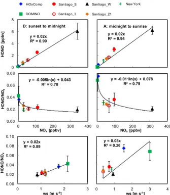
3.2.1 Nighttime HONO levels

In contrast to daytime HONO levels, which are generally higher than expected based on model calculations (e.g., Kleffmann et al., 2005; Acker et al., 2006; Li et al., 2010; S ¨orgel et al., 2011a; Su et al., 2011; Elshorbany et al., 2012), HONO concentrations

10

during nighttime can be largely explained by known sources, i.e., the heterogeneous reaction on humid surfaces (Alicke et al., 2002) and direct emissions (Vogel et al., 2003). All measurement campaigns are included in this analysis except MCMA-2006, for which no nighttime HONO data are available. Though the correlation between HONO and NOx during both night sectors, A and D, reveal a similar slope of about 15

0.02 (see Fig. 4), the HONO/NOx ratio itself is found to to be logarithmically related

to NO_x, which can be explained by the nighttime heterogeneous formation of HONO (Kleffmann et al., 2003). This is confirmed by the HONO/NOx dependency on wind

speed (ws) (see Fig. 4). In addition, the slope of the HONO/NOxratio versus NOxwas

found to be about two times higher in sector A compared to sector D (see Fig. 4),

20

resulting in the following two regression equations:

[HONO]A=((−0.011±0.002) ln([NO_x])+(0.078±0.009))×[NO_x] (1)

[HONO]D=((−0.005±0.001) ln([NOx])+(0.043±0.004))×[NOx] (2)

Similarly, anti-correlation between HONO/NOx ratio and NOx was previously reported

(S ¨orgel et al., 2011b). Again, for the correlation between HONO/NOxratio and ws, the 25

slope in sector A is higher than that in sector D, albeit with a higher correlation co-e_fficient in sector D (see Fig. 4). Nevertheless, as shown in Fig. 5, simulated HONO

(12)

ACPD

12, 12885–12934, 2012

chemistry

Title Page

Tables Figures

◭ ◮

Back Close

Full Screen / Esc

Discussion

P

a

per

|

Dis

cussion

P

a

per

|

Discussion

P

a

per

|

Discussio

n

P

a

per

|

using Eqs. (1) and (2) (sector A and D, respectively) is only improved for measure-ment campaigns with a nighttime HONO/NO_xratio>0.02, i.e., HOxComp, Santiago S and DOMINO, compared to that using the mean HONO/NOx ratio of 0.02, while for

other campaigns, measured HONO was reasonably well simulated based on the mean HONO/NO_xratio of 0.02.

5

3.2.2 Daytime HONO mixing ratio

During daytime, a similar regression slope of 0.02±0.002 between measured HONO and NO_xmixing ratio was obtained for all measurement campaigns (see Fig. 6), albeit with a lower correlation coefficient in comparison to nighttime values, which is mainly due to the low correlation between HONO and NOx during the afternoon (sector C, 10

see below). However, in contrast to nighttime, the HONO/NOx ratio during daytime is

independent of HONO and NO_x mixing ratios while it has a light dependency (given byj(NO2), though with a low correlation coefficient (R

2

=0.23). These results are in agreement with Zhang et al. (2012), who showed that the daytime HONO flux does not correlate significantly with measured NO_x mixing ratios, suggesting that under these

15

conditions NOx is not an important precursor of HONO daytime formation. In

addi-tion, using the Community Multiscale Air Quality (CMAQ) model, Czader et al. (2012) demonstrated that photochemical HONO formation can be a strong source during day-time, which directly impacts HOx and ozone levels.

During daytime, HONO mixing ratios are controlled by the photostationary state

con-20

centration of HONO, [HONO]pss, calculated from the known gas phase chemistry by the following equation:

[HONO]pss= kOH+NO[OH][NO]

j(HONO)+kOH+HONO[OH]

(3)

plus other sources that are not known or not accounted for, henceforth denoted as “unidentified”. Owing to their negligible contributions during daytime, heterogeneous

25

(13)

ACPD

12, 12885–12934, 2012

chemistry

Title Page

Tables Figures

◭ ◮

Back Close

Full Screen / Esc

Discussion

P

a

per

|

Dis

cussion

P

a

per

|

Discussion

P

a

per

|

Discussio

n

P

a

per

|

S ¨orgel et al., 2011a) are ignored. Given the reported low HONO/NO_x ratio of 0.3– 0.8 % for directly emitted HONO estimated at a NO/NOx ratio of >0.9 (Kurtenbach

et al., 2001), and considering the variable low NO/NOxratios (0.2 to 0.6) and the much

higher measured HONO/NO_x ratios for the investigated campaigns, emitted HONO contributions are not expected to contribute significantly to measured HONO levels (Su

5

et al., 2008) during the investigated campaigns and are therefore not considered in the following calculation. For the estimation of [HONO]pss the OH concentration and the HONO photolysis frequency (j(HONO)) in addition to measurements of NO and HONO mixing ratios are required, which were available only for four measurement campaigns, HOxComp, Santiago S, Santiago W and DOMINO. For all campaigns [HONO]pss was

10

calculated using the IUPAC recommendations (Atkinson et al., 2004). During daytime [HONO]pss constituted 29, 72, 55 and 50 % of measured HONO levels during HOx-Comp, Santiago S, Santiago W and DOMINO, respectively. Unidentified HONO mix-ing ratios were calculated by subtractmix-ing the calculated [HONO]pss from the measured HONO mixing ratios. The largest contributions of [HONO]pss are typically obtained

15

during the early morning (sector B, from sunrise to mid-noon) reaching a maximum during the rush hour.

As shown in Fig. 7, high correlations were obtained between average HONO, [HONO]pss and unidentified HONO mixing ratios versus NO_xlevels for the investigated measurement campaigns during both, sector B and daytime (sectors B+C). However,

20

the regression slopes for the measured HONO and unidentified HONO levels versus NO_xwere higher during daytime in comparison to that of sector B, showing that uniden-tified sources contribute most during the afternoon, again in good agreement with pre-vious studies, which showed that the high afternoon HONO/NOx ratio points towards

an unknown HONO daytime sources (e.g., Kleffmann et al., 2005; Elshorbany et al.,

25

2009a, 2010b, 2012). Consequently, a higher correlation coefficient was obtained for the relationship between HONO, [HONO]pss and NOx during sector B in comparison

to the average daytime values. In contrast, for [HONO]pss, similar slopes were ob-tained during daytime as well as sector B, implying similar average contributions (i.e.,

(14)

ACPD

12, 12885–12934, 2012

chemistry

Title Page

Tables Figures

◭ ◮

Back Close

Full Screen / Esc

Discussion

P

a

per

|

Dis

cussion

P

a

per

|

Discussion

P

a

per

|

Discussio

n

P

a

per

|

of [HONO]pss to HONO measured mixing ratios) during both sectors, B and C. For sector B, the following linear regression expressions were obtained:

[HONO]pss=(0.014±0.001)×[NOx] (4)

[HONO]B=(0.021±0.001)×[NOx] (5)

As shown in Fig. 5, HONO mixing ratios in sector B calculated by Eq. (5) and by the

5

global mean of 0.02 are similar and in very good agreement with that measured, related to the similar slope of HONO/NOxin sector B and the mean HONO/NOx ratio of 0.02,

except for Santiago 3, Santiago 21 and MCMA-2006. In fact, measured HONO during sector B for Santiago 21 and Santiago 3 could have been accurately simulated based on Eq. (4) alone, which shows that measured HONO during sector B in these data sets

10

can be largely explained by [HONO]pss. However, for consistency we used Eq. (5) for sector B in all data sets. For MCMA-2006, the overestimation of HONO mixing ratios in sector B is due to the very high measured NOxmixing ratio, which is not related to that

of HONO (see below).

The noon to sunset time period (sector C) is the most important one in the HONO

15

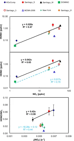
diurnal profile, during which unidentified daytime HONO sources contribute most sig-nificantly. The linear regression analysis for this time period was found to result in two different slopes as shown in Fig. 8 (middle panel). For measurement campaigns with a HONO/NO_x ratio of ≤0.02, i.e., DOMINO, Santiago 3, Santiago 21, New York and

MCMA-2006, a high correlation is obtained with a regression slope of 0.017±0.003,

20

while measurement campaigns with a HONO/NOx ratio>0.02, i.e., HOxComp,

Santi-ago S, SantiSanti-ago W indicate a regression slope of 0.042±0.01 (Fig. 8, middle panel).

The regression slope for measurement campaigns with HONO/NOx ratios ≤0.02 is

quite comparable to that of [HONO]pss vs. NOx (see Fig. 7), which shows that HONO

mixing ratios during this time period for these measurement campaigns can be

de-25

scribed accurately by [HONO]pss, with an additional small contribution from unidenti-fied sources. Interestingly, a very high correlation (R2=0.99) between the HONO/NOx

(15)

ACPD

12, 12885–12934, 2012

chemistry

Title Page

Tables Figures

◭ ◮

Back Close

Full Screen / Esc

Discussion

P

a

per

|

Dis

cussion

P

a

per

|

Discussion

P

a

per

|

Discussio

n

P

a

per

|

ratios>0.02 (see Fig. 8), from which HONO mixing ratios during sector C can be cal-culated as:

[HONO]C=(9.42±0.16)×j(NO₂)×[NO_x] (6)

For those with a HONO/NOx ratio≤0.02, a much worse correlation (R 2

=0.44), even with a negative slope was obtained. Consequently, for measurement campaigns with

5

HONO/NO_x ratios>0.02, calculated HONO mixing ratios based on the above Eq. (6) match the measurements well (see Fig. 5), while for those with a HONO/NOx ratio ≤0.02, measured HONO mixing ratios are better simulated using the average of 0.02. One potential explanation for this differentj(NO₂) dependency is that for measurement campaigns with a HONO/NOxratio≤0.02, unknown daytime HONO sources that are 10

j(NO2) dependent do not contribute significantly to the measured HONO mixing ratios.

Indeed, for two of these measurement campaigns, DOMINO and New York, unidenti-fied daytime HONO source strengths of about 100 and 150 pptv h−1, respectively were reported, which is very low compared to that of about 0.33, 1.7 and 2.5 ppbv h−1 for HOxComp, Santiago S and Santiago W, respectively. Similarly, the unknown source

15

strengths for other campaigns reported in the literature are also in the range of 200– 500 pptv h−1, 500 pptv h−1 and up to 2 ppbv h−1 calculated for rural, semi-urban and urban conditions, respectively (Kleffmann et al., 2007). For MCMA-2006, an additional daytime HONO source was reported (Dusanter et al., 2009) despite the low average daytime HONO/NOx ratio of about 0.01. However, as mentioned above (Sect. 2.2), 20

this is due to the different spatial account of HONO and NO_x (i.e., measuring diff er-ent air masses of HONO and NOx). During MCMA-2006 HONO was measured using

an LP-DOAS system over an optical path length of 5285 m while NOx was measured

using a local commercial standard instrument, which is known to be affected by inter-ferences from other NOy components (e.g., HNO3, PAN, RNO3, etc.). Therefore, the 25

low HONO/NOx ratio of 0.01 is likely to be caused by higher measured NOx levels

in different air masses. Unfortunately, no strict method or correlation could be found to predict the HONO/NO_xratio (i.e.,>0.02 or≤0.02). Therefore the di_fferent dependency

(16)

ACPD

12, 12885–12934, 2012

chemistry

Title Page

Tables Figures

◭ ◮

Back Close

Full Screen / Esc

Discussion

P

a

per

|

Dis

cussion

P

a

per

|

Discussion

P

a

per

|

Discussio

n

P

a

per

|

of HONO/NO_xonj(NO₂) can only be used as an indicator of the presence of significant unknown HONO sources, rather than to predict the HONO concentration.

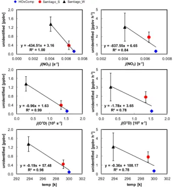
3.2.3 Unidentified HONO sources

The contribution of unidentified HONO sources to measured HONO during the after-noon (sector C, from after-noon to sunset) was largest during HOxComp (∼91 %) followed 5

by Santiago W (∼69 %) and Santiago S (∼25 %). As shown in Fig. 9, high correla-tions are obtained between unidentified HONO mixing ratios and their derived source strength (ppb h−1) withj(NO₂),j(O1D) and temperature for sector C. The good agree-ment for both j(NO₂) and j(O1D) relates to the onsets of sunrise and sunset being defined at 30 % of the maximumj(NO2) values, when thej(O

1

D) values correspond

10

to about 10 % of their daytime maximum. This method allows investigating the depen-dency of unidentified daytime HONO sources on both,j(NO₂) andj(O1D). In previous studies (e.g., Elshorbany et al., 2009a, 2012), better agreement was obtained for the correlation between unidentified HONO sources andj(NO2) in comparison toj(O

1

D) by considering the full photolysis frequency range of these photolysis rates, and the

15

latter produces an intercept due to the smaller span of j(O1D). However, the good correlation between unidentified HONO sources (see Fig. 9) and temperature (in addi-tion toj(NO₂) andj(O1D)) implies that photolytic sources active at longer wavelengths (e.g., photosensitized conversion of NO2 on organic surfaces, Stemmler et al., 2006)

or photolysis of nitro aromatic compounds (Bejan et al., 2006) or those that arej(O1D)

20

dependent, e.g., the photolysis of HNO3 (Zhou et al., 2003, 2011) or those that are

temperature dependent (Su et al., 2011), are all of significance. Despite that these results leave the question of unknown HONO daytime sources open, they offer linear regression equations that can be used as an indicator for unknown HONO production within the range of conditions investigated (i.e., at a HONO/NO_xratio>0.02).

25

Interestingly, the unidentified HONO sources were found to correlate inversely with

j(NO2), j(O

1

(17)

ACPD

12, 12885–12934, 2012

chemistry

Title Page

Tables Figures

◭ ◮

Back Close

Full Screen / Esc

Discussion

P

a

per

|

Dis

cussion

P

a

per

|

Discussion

P

a

per

|

Discussio

n

P

a

per

|

showed that nocturnal HONO mixing ratios directly correlate to radon, especially in winter. He also measured the highest HONO mixing ratios of 2.4 ppb at night in Jan-uary (1999) coinciding with very high radon levels. Thus, Veitel (2002) concluded that surfaces at or near the ground form the most prominent HONO source both by day and night. Similarly, Febo et al. (1999) stated that especially trace gases emitted or formed

5

near the ground show a direct and strong correlation with radon. The correlations in Fig. 9 are also quite interesting because they show that unidentified HONO sources during afternoon can be directly calculated as a function ofj(NO2) orj(O

1

D) (also vs. temperature but with less accuracy) as follows:

Unidentified HONO (ppbv h−1₎

=(−838±360)j(NO₂)+(6.65±2.15) , (7) 10

Unidentified HONO (ppbv h−1₎

=(−1.78±0.94)×105j(O1D) (8)

Indeed, considering an estimated daytime average j(NO2) for Xinken, China

(PRIDE PRD2004) and Back Garden, China (PRIDE-PRD2006) of about 0.005 and 0.007 s−1, the approximate unidentified HONO source strength based on the relation-ship Eq. (7) would be about 2.5±1.1 and 0.78±0.34 ppb h−1, respectively which is in

15

good agreement with those reported by Li et al. (2012). Nevertheless, since the above correlations were derived based on a limited number of measurement campaigns, fur-ther evaluation is required.

3.2.4 Measured vs. simulated HONO levels

Figure 10 shows the correlations between measured and simulated HONO mixing

ra-20

tios based on Eqs. (1) to (6) and the mean HONO/NOx ratio of 0.02 for all

investi-gated measurement campaigns. It appears that measured HONO diurnal profiles for all campaigns can be simulated quite well for both 24 h and daytime averages with a linear measured/simulated regression slope of 1.10±0.05 and 0.91±0.07, respec-tively. Similar agreement is also obtained between measured and calculated HONO

25

mixing ratios using the mean HONO/NOxratios of 0.02 with slopes of 1.02±0.05 and

1.06±0.13, respectively, albeit with lower correlation coe_fficients, which is due to the

(18)

ACPD

12, 12885–12934, 2012

chemistry

Title Page

Tables Figures

◭ ◮

Back Close

Full Screen / Esc

Discussion

P

a

per

|

Dis

cussion

P

a

per

|

Discussion

P

a

per

|

Discussio

n

P

a

per

|

underestimation of measured HONO mixing ratios during the afternoon for measure-ment campaigns with HONO/NOxratios>0.02 (see Sect. 3.2.2). This can only be

ac-counted for by Eq. (6). However, the calculation of afternoon HONO mixing ratios using Eq. (6) requires the prior knowledge of the HONO/NO_x ratio (see Sect. 3.2.2), which is not feasible for a prognostic method. In addition, during daytime the slope of the

re-5

lationship between HONO and NOx for all measurement campaigns is 0.022±0.002,

which is quite similar to the overall mean HONO/NO_xratio. Therefore, the overall mean HONO/NOx ratio of 0.02 is considered to be most suitable to approximate the HONO

mixing ratios and investigate the global impact of HONO photolysis during daytime on HO_xand O₃chemistry.

10

3.3 Global impact

In global models HONO is typically simulated based on the known gas phase chem-istry, thus only accounting for [HONO]pss (see Sect. 3.2.2) rather than observed HONO, thus significantly underestimating ambient concentrations. Consequently, HO_x, O3and other secondary oxidation products from HONO photolysis during daytime are 15

also expected to be significantly underestimated. Since most polluted regions with high NO_x levels are located in the Northern Hemisphere, the impact of using more realistic HONO levels should be most pronounced in this part of the world, where NO levels are often sufficient for efficient radical recycling (Lelieveld et al., 2002; Elshorbany et al., 2010b). To investigate the impacts by HONO photolysis, including the seasonal

depen-20

dency, we focus on model output for the months June and December. The global mean HONO/NOxratio of 0.02, empirically derived from the correlation between HONO and

NOx has been implemented in the EMAC model. In addition, the sensitivity runs S1

and S3 apply di_fferences by a factor of two, thus using a HONO/NO_xratios of 0.01 and 0.04, respectively.

25

As shown in Fig. 11, simulated HONO levels based on a HONO/NOx ratio of 0.02

(19)

ACPD

12, 12885–12934, 2012

chemistry

Title Page

Tables Figures

◭ ◮

Back Close

Full Screen / Esc

Discussion

P

a

per

|

Dis

cussion

P

a

per

|

Discussion

P

a

per

|

Discussio

n

P

a

per

|

These results are in agreement with Li et al. (2010), Zhang et al. (2011) and Czader et al. (2012) who showed that measured HONO mixing ratios are about tenfold of those calculated when this reaction is the only formation mechanism. The simulated HONO levels in the S2 run in December are higher than those during June, which is also good agreement with previous studies, showing that HONO levels in winter are higher

5

than in summer (e.g., Elshorbany et al., 2010a). The simulated HONO levels in June in South Korea and in December in East China compare well to those measured during May–July 2005 in Seoul (Korea) and during October–January 2004/2005 in Shanghai (China) (Li et al., 2012, and references therein).

Figure 12 shows that the shape of the simulated diurnal HONO profile on 10 July,

10

2005, in North-West Germany (50.93◦N, 6.36◦E) using the base model, di_ffers strongly from the observations during the HOxComp and other campaigns presented in Fig. 1. Owing to the coarse spatial resolution of the model the profiles in Fig. 12 represent larger areas than the measurements, though the agreement is rather good, probably indicating that HOxComp is representative of this area. In contrast to the base

sce-15

nario, the shape of the simulated HONO diurnal profiles, S1, S2 and S3 based on the HONO/NO_xratios of 0.01, 0.02 and 0.04, respectively match the measurements much better with maximum HONO mixing ratios during the early morning and minimum val-ues during afternoon. The simulated HONO by the S2 run (based on a HONO/NOxratio

of 0.02) agrees best with the measurements. These results corroborate our earlier

con-20

clusion that simulating HONO based on a mean HONO/NOxratio of 0.02 provides a

re-alistic representation of HONO, rather than considering only the gas phase formation of HONO. Therefore, the S2 run is used hereafter to investigate the impact of imple-menting this more realistic HONO profile. As also shown in Fig. 12, enhancements in OH, HO2, O3, PAN, H2O2, NOx and HNO3 are calculated only at NO levels of about 25

1 ppbv (marked by the dashed line in the diurnal NO profile). When NO levels are below 1 ppbv, enhancements are typically small or negligible. This is due to the low recycling efficiency (under NO sensitive conditions), under which any increase in the OH levels as a result of HONO photolysis does not lead to a significant increase in the HO₂levels

(20)

ACPD

12, 12885–12934, 2012

chemistry

Title Page

Tables Figures

◭ ◮

Back Close

Full Screen / Esc

Discussion

P

a

per

|

Dis

cussion

P

a

per

|

Discussion

P

a

per

|

Discussio

n

P

a

per

|

from reaction (RO₂+NO→HO₂) or H₂O₂from the reaction of (HO₂+HO₂→H₂O₂) or

O3from the reaction of (RO2/HO2+NO→O3). These results show that an increase in

the HOx levels as well as in the secondary oxidation products only occurs under

con-ditions of efficient recycling of OH through RO₂/HO₂, in agreement with the sensitivity analysis performed for HOxComp (Elshorbany et al., 2012). The enhancement of HOx 5

as a result of applying higher HONO values also leads to a redistribution of model calculated reactive nitrogen compounds. For example, the increased levels of OH, HO2 and other secondary oxidation products (e.g., acyl peroxy radicals (RC(O)O2))

may reduce NO2 (e.g., OH+NO2→HNO3, RC(O)O2+NO2→PAN) and NO (e.g.,

HO₂+NO→OH+NO₂) forming HNO₃ and PAN. As shown in Fig. 12, the additional 10

daytime HONO leads to a decrease in NO and NO₂, while HNO₃ and PAN increase during the high NOx period. During daytime (6:00 – 18:00 UTC), NO, NO2, OH, HO2,

O3, PAN, H2O2and HNO3change by−19,−9, 36, 45, 10, 26, 2 and 19 %, respectively

in the S2 run compared to the base model, in agreement with previous studies (e.g., Li et al., 2011).

15

To further investigate the impact of the more realistic HONO levels in relatively pol-luted areas (high-NO_x, VOC-limited conditions), Fig. 13 compares the simulated diurnal profiles in the Eastern USA and downwind on 1 June 2005. It appears that the shape of the simulated diurnal HONO profiles from the runs S1, S2 and S3 match very well those measured in field campaigns (see Fig. 1), in contrast to that simulated using the

20

base scenario. As shown in Fig. 13, significant increases in HOx and the secondary

oxidation products result from the more realistic HONO levels (simulated by S2). Un-fortunately, no HONO field measurements are available for comparison in this area for 2005. The simulated maximum O3 levels (S2) agree with the reported levels in New

York State in 2005 (New York State Department of Environmental Conservation).

Sim-25

ilar to the HOxComp case, NO and NO₂ decrease while HO_x, O₃, PAN, H₂O₂ and HNO3 increase, with higher relative enhancements compared to HOxComp, owing to

(21)

ACPD

12, 12885–12934, 2012

chemistry

Title Page

Tables Figures

◭ ◮

Back Close

Full Screen / Esc

Discussion

P

a

per

|

Dis

cussion

P

a

per

|

Discussion

P

a

per

|

Discussio

n

P

a

per

|

These results underscore that the more realistic representation of HONO in a global model leads to an enhancement in simulated HOx and oxidation products,

predomi-nantly under high NOxconditions.

Figures 14 and 15 show the absolute and relative enhancements, respectively, in OH and O3 together with simulated NO levels. As shown in Fig. 14, in the relatively 5

polluted Northern Hemisphere average monthly NO mixing ratios in December are typically two times higher than in June. In addition, in June NO levels are relatively high in the Northeastern USA and in Northern Europe, e.g., in comparison to Eastern China. Consequently, the enhancements of OH and O3 levels are relatively strong in

these high-NO_x regions. Also, over Eastern China in December where NO levels are

10

higher than in the USA and Europe, the enhancements of OH and O₃levels are larger. In addition, the relative enhancements of OH and O3 are significantly higher in the

winter hemispheres compared to summer (see Fig. 15). Similarly, previous studies showed that the impact of HONO photolysis on OH is higher in winter than in summer (Aumont, 2003; Elshorbany et al., 2010a), owing to the relatively minor importance of

15

the other photochemical sources such as O3 and HCHO (Elshorbany et al., 2010b),

in addition to the higher NO levels in winter. Thus, the increased HONO levels in the model significantly enhance the oxidation capacity in polluted regions, especially in winter, when other photolytic OH sources are of minor importance.

Figures 16 and 17 show some details of the model calculated enhancement in

20

OH, O3, NOx, HNO3 and PAN over the Eastern USA in June and Eastern China in

December, together with the NO mixing ratios (top panels in Fig. 16). It is evident that the relative enhancements in these species follow the relative changes in NO. In these high-NOxregions, monthly average OH enhancements up to about 1.5×10

6

and 0.6×106mol cm−3are calculated for June and December 2005, respectively, while O3 25

is calculated to increase up to 12 and 8.5 ppbv, respectively. These increases are highly significant, corresponding to relative OH and O3enhancements of about 80 and 30 %

in June and about 90 and 40 % in December, respectively. These results are quite similar to those of previous studies for specific locations applying local models. For

(22)

ACPD

12, 12885–12934, 2012

chemistry

Title Page

Tables Figures

◭ ◮

Back Close

Full Screen / Esc

Discussion

P

a

per

|

Dis

cussion

P

a

per

|

Discussion

P

a

per

|

Discussio

n

P

a

per

|

example, model simulations of daytime HONO in Mexico City, which could only achieve about 30–50 % of the observed HONO, indicate an average midday O3enhancement of

6 ppbv (Li et al., 2010). Similarly, Li et al. (2011) reported an average O3enhancement

of 12 ppbv (∼50 %) compared to the base case considering only gas phase HONO

formation. These results are also in good agreement with Elshorbany et al. (2009b)

5

who compared box model calculations constrained by measured HONO to those only considering OH+NO→HONO. In the latter case, O₃levels decreased on average by

30 % during daytime. Similarly, Harris et al. (1982) and Clapp and Jenkin (2001), em-ploying photochemical trajectory models, showed that HONO photolysis may have an important impact on the level of oxidants mostly under polluted high-NO_x conditions.

10

Jorba et al. (2012) also showed that O₃levels are enhanced in response to additional OH production only in high-NOx regions though can be decreased in regions with

low-NOxconditions.

These results illustrate that because of the bu_ffering e_ffect by NO_x the mean HONO/NOxratio is a reasonable proxy to simulate HONO levels in global models, thus 15

avoiding severe underestimation of HONO concentrations, with consequences for sim-ulated HO_xand secondary oxidation products. In the view of the many unknowns and uncertainties about daytime HONO sources, global models could apply this method until the chemistry of HONO is resolved in greater detail.

4 Conclusions

20

HONO, NOx and auxiliary atmospheric chemistry parameters have been investigated

using data from 15 field measurement campaigns around the globe (from 52◦N to 37◦S and from 116◦E to 99◦W). The high correlation between HONO and NO_x in all data sets reveals a robust and consistent linear regression slope of 0.02±0.002. Our analysis indicates that, given the ambient NOx mixing ratio, the HONO/NOx ratio is 25

(23)

ACPD

12, 12885–12934, 2012

chemistry

Title Page

Tables Figures

◭ ◮

Back Close

Full Screen / Esc

Discussion

P

a

per

|

Dis

cussion

P

a

per

|

Discussion

P

a

per

|

Discussio

n

P

a

per

|

For nighttime conditions, we derive a linear regression slope of 0.02±0.001 based

on all investigated campaigns. The HONO/NO_x ratio itself was appear to have a loga-rithmic relationship with NOx, which can be explained by the nighttime heterogenous

formation of HONO. This is corroborated by the HONO/NOx dependence on wind

speed. In addition, the regression slope of the HONO/NO_x ratio versus NO_x is

dif-5

ferent during both nighttime sectors A (midnight to sunrise) and D (sunset to midnight), from which the HONO concentration can be calculated as a function of NOxlevels.

During daytime, a similar regression slope of 0.02±0.002 between measured HONO

and NOx mixing ratios is obtained for all investigated measurement campaigns.

How-ever, in contrast to nighttime conditions, the HONO/NOxratio is independent of HONO 10

and NO_x mixing ratios, in agreement with previous studies. The correlations between [HONO]pss and NOxduring time sector B (sunrise to noon) as well as during daytime

(time sectors B+C) reveal a similar correlation slope of 0.014, implying comparable contributions during both time sectors B and C. In contrast, the correlations between unidentified HONO and NOxmixing ratios during the time sector B reveal a regression 15

slope of 0.007, much lower than the 0.011 obtained for daytime, implying higher contri-butions by unidentified sources during the afternoon, also in agreement with previous studies. In contrast to time sector B, the correlation between HONO and NOx during

sector C (noon to sunset) results in two different correlation slopes. For measurement campaigns with HONO/NO_x ratios ≤0.02, a regression slope of 0.017±0.003 is ob-20

tained, while measurement campaigns with HONO/NOx ratios>0.02 follow a

regres-sion slope of 0.042±0.01. These results imply that for conditions with HONO/NOx

ratios≤0.02, HONO mixing ratios during time sector C can be largely represented by

[HONO]pss, with small additional contributions by unidentified sources. A very high cor-relation (R2=0.99) between the HONO/NOxratio andj(NO2) is obtained only for con-25

ditions with a HONO/NO_x ratio >0.02, while for those with HONO/NO_x ratios ≤0.02,

a much worse correlation (R2=0.44), even a negative slope is obtained. A potential ex-planation for this differentj(NO2) dependency is that during measurement campaigns

(24)

ACPD

12, 12885–12934, 2012

chemistry

Title Page

Tables Figures

◭ ◮

Back Close

Full Screen / Esc

Discussion

P

a

per

|

Dis

cussion

P

a

per

|

Discussion

P

a

per

|

Discussio

n

P

a

per

|

with HONO/NO_x ratios ≤0.02, unknown daytime HONO sources that are j(NO₂)

de-pendent do not contribute significantly.

High correlations are also obtained between unidentified HONO and its source strength (ppb h−1), and j(NO₂), j(O1D) and temperature for time sector C (noon to sunset). These results imply that photolytic sources active at longer wavelengths or

5

those that arej(O1D) dependent are of significance. In fact these results suggest that sources that are solely temperature dependent may also be important, as predicted by Su et al. (2011). Interestingly, we also find that unidentified HONO sources correlate inversely withj(NO2),j(O

1

D) and temperature, from which they can be estimated. The mean HONO/NO_xratio of 0.02, derived from all measurement campaigns

inves-10

tigated, has been implemented into the EMAC chemistry-climate model to calculate the global HONO distribution. Strong HONO enhancements are predicted relative to the base model, which only accounts for the gas phase reaction of OH with NO. Rea-sonable agreement is obtained between simulated and measured HONO mixing ratios during both summer and winter. The simulated HONO mixing ratios appear to have

15

a significant impact on HOx, O3 and other oxidants, however, predominantly under

polluted high-NO_xconditions. Furthermore, the relative enhancements in OH and sec-ondary products were higher in winter than in summer, thus enhancing the oxidation capacity in polluted regions, especially in winter, when the other photolytic OH sources are of minor importance. The results of the current study suggest that realistic HONO

20

levels should be accounted for by global models and that simulated HOx, O3and

sec-ondary oxidation products should be revised accordingly.

Acknowledgements. The authors would like to thank J. Kleffmann, S. Dusanter, X. Ren and M

S ¨orgel for kindly supplying their measurement data for their measurement campaigns namely, Santiago de Chile (2009), MCMA-2006, New York and DOMINO, respectively. The research 25

(25)

ACPD

12, 12885–12934, 2012

chemistry

Title Page

Tables Figures

◭ ◮

Back Close

Full Screen / Esc

Discussion

P

a

per

|

Dis

cussion

P

a

per

|

Discussion

P

a

per

|

Discussio

n

P

a

per

|

The service charges for this open access publication have been covered by the Max Planck Society.

References

van Aalst, M. K., van den Broek, M. M. P., Bregman, A., Br ¨uhl, C., Steil, B., Toon, G. C., Garcelon, S., Hansford, G. M., Jones, R. L., Gardiner, T. D., Roelofs, G. J., Lelieveld, J., 5

and Crutzen, P. J.: Trace gas transport in the 1999/2000 Arctic winter: comparison of nudged GCM runs with observations, Atmos. Chem. Phys., 4, 81–93, doi:10.5194/acp-4-81-2004, 2004.

Acker, K., M ¨oller, D., Wieprecht, W., Meixner, F. X., Bohn, B., Gilge, S., Plass-D ¨ulmer, C., and

Berresheim, H.: Strong daytime production of OH from HNO₂at a rural mountain site,

Geo-10

phys. Res. Lett., 33, L02809, doi:10.1029/2005GL024643, 2006.

Alicke, B., Platt, U., and Stutz, J.: Impact of nitrous acid photolysis on the total hydroxyl radical budget during the limitation of oxidant production/pianura padana produzione di ozono study in Milan, J. Geophys. Res., 107, 8196, doi:10.1029/2000JD000075, 2002.

Alicke, B., Geyer, A., Hofzumahaus, A., Holland, F., Konrad, S., P ¨atz, H. W., Sch ¨afer, J., 15

Stutz, J., Volz-Thomas, A., and Platt, U.: OH formation by HONO photolysis during the BERLIOZ experiment, J. Geophys. Res., 108, 8247, doi:10.1029/2001JD000579, 2003. Atkinson, R., Baulch, D. L., Cox, R. A., Crowley, J. N., Hampson, R. F., Hynes, R. G.,

Jenkin, M. E., Rossi, M. J., and Troe, J.: Evaluated kinetic and photochemical data for

at-mospheric chemistry: Volume I – gas phase reactions of O_x, HO_x, NO_x and SO_x species,

20

Atmos. Chem. Phys., 4, 1461–1738, doi:10.5194/acp-4-1461-2004, 2004.

Aumont, B., Chervier, F., and Laval, S.: Contribution of HONO sources to the NO_x/HO_x/O₃

chemistry in the polluted boundary layer, Atmos. Environ., 37, 487–498, 2003.

Bejan, I., Abd El Aal, Y., Barnes, I., Benter, T., Bohn, B., Wiesen, P., and Kleffmann, J.: The

photolysis of ortho-nitrophenols: a new gas phase source of HONO, Phys. Chem. Chem. 25

Phys., 8, 2028–2035, doi:10.1039/b516590c, 2006

Br ¨uhl, C., Lelieveld, J., Crutzen, P. J., and Tost, H.: The role of carbonyl sulphide as a source of stratospheric sulphate aerosol and its impact on climate, Atmos. Chem. Phys., 12, 1239– 1253, doi:10.5194/acp-12-1239-2012, 2012.