*e-mail: [email protected]
Experimental Analysis and Theoretical Predictions of the Limit Strains
of a Hot-dip Galvanized Interstitial-free Steel Sheet
Maria Carolina dos Santos Freitasa, Luciano Pessanha Moreiraa∗, Renata Garcez Vellosob
aPrograma de Pós-graduação em Engenharia Metalúrgica, Universidade Federal Fluminense – UFF, Av. dos Trabalhadores, 420, CEP 27255-125, Volta Redonda, RJ, Brazil
bCompanhia Siderúrgica Nacional, Rod. BR 393, Km 5, 001, CEP 27260-390, Volta Redonda, RJ, Brazil
Received: August 3, 2012; Revised: November 6, 2012
In this work, the formability of a hot-dip galvanized interstitial-free (IF) steel sheet was evaluated by means of uniaxial tensile and Forming Limit Curve (FLC) tests. The FLC was defined using the flat-bottomed Marciniak’s punch technique, where the strain analysis was made using a digital image correlation software. A plastic localization model was also proposed wherein the governing equations are solved with the help of the Newton’s method. The investigated hot-dip galvanized IF steel sheet presented a very good formability level in the deep-drawing range consistent with the measured Lankford values. The predicted limit strains were found to be in good agreement with the experimental data of the hot-dip galvanized IF steel sheet owing to the definition of the localization model geometrical imperfection as a function of the experimental surface roughness evolution and, in particular, to the yield surface flattening near to the plane-strain stress state authorized by the adopted yield criterion.
Keywords: IF steel, modeling, forming limit curve, sheet-metal forming
1. Introduction
The concept of the Forming Limit Diagram (FLD) was introduced by Keeler1 in order to assess the formability of
sheets under biaxial tension. This earlier study applied for positive values of the smaller principal strain in the plane of the sheet. It was next extended by Goodwin2 to the full range
between uniaxial and equibiaxial tension. Since that time, a very large number of investigations have been devoted to the experimental determination and the theoretical modeling of limit strains in sheets under biaxial tension. The FLD is defined in the axes of minor and major principal strains in the plane of the sheet. The curve obtained by plotting the limit strains obtained for linear strain paths is the Forming Limit Curve (FLC). The FLC is commonly observed to be fairly independent of the test used for its determination, provided the strain paths remain almost linear up to the occurrence of intense flow localization. More generally, the limit strains are assumed by most researchers to represent an intrinsic, although strain-path dependent, property of the material. In other words, structural effects relating to the boundary conditions of the deformation process are implicitly assumed to be without influence on the limit strains.
The prediction of the forming limits set by the occurrence of localized necking in plastically stretched sheets has been the subject of a very large number of theoretical analyses. The most popular approach is based on the model originally proposed by Marciniak and Kuczynski3. This approach,
hereafter referred to as the M-K model, assumes the existence of an initial thickness imperfection across the sheet. Afterwards, the forming limits result from the process of flow
localization in the defective region. Almost all the available descriptions of plastic yielding have been implemented in such a simple plane-stress analysis involving the existence of two individual zones, namely, the homogeneous zone, and the defective, thinner zone. In addition to the beneficial effects of strain-hardening and strain-rate hardening to delay the development of the neck4,5, it is now well established that
the forming limits strongly depend on the plasticity model adopted, and in particular on the shape of the yield surface6-8.
Thus, considerable advances have been achieved during the last twenty years in the prediction of the sheet metal forming limits by employing yield criteria proposed to provide an improved description of plastic flow under conditions of biaxial loading. For instance, predictions in good agreement with experimental results have been obtained in the case of aluminum alloys9-10 with the yield criteria proposed by
Barlat et al.11, Karafillis and Boyce12 and Barlat et al.13.
The effects of the through-thickness normal and shear stress components have also been taken into account within the framework of the M-K model, see the recent works14-18. These out-of-plane effects are
not negligible in some sheet metal forming processes, such as hydroforming and incremental sheet forming, where significant through-thickness compressive stress components may take place.
in sheet thickness (geometric imperfection) was amended by considering also possible variations in the strength of the material (material or metallurgical imperfection). This idea was already mentioned in the work of Marciniak et al.19,
and it was later materialized by assuming spatial variations in the orientation distribution of grains, giving variations in the Taylor factor20. Inhomogeneous damage due to the
nucleation and growth of microvoids can also occur, for instance by decohesion between matrix and inclusion, or by fragmentation of inclusions, leading to a decrease in the surface area transmitting the load21. Indeed, the flow
localization process in the presence of an initial thickness imperfection is accelerated by the development of damage, which is more rapid in the thinner, more stretched region22,23.
A quasi-random arrangement of hard elastic inclusions was also considered in finite element (FE) calculations to generate inhomogeneous strain fields leading to necking of the representative volume element24,25. Wu et al.26 performed
FE computations of the response of a macroscopically infinitely small unit cell made of an assembly of elements, where each element represents a grain following the constitutive laws of crystal plasticity. The orientation distribution of grains is representative of a given texture. Then, the flow localization process can be analyzed at this mesoscopic level under a given average stress-ratio, and compared with the M-K analysis results.
The present work aims at evaluating first the formability of a hot-dip galvanized interstitial-free steel sheet using the Marciniak flat-bottomed punch test technique, where the limit strains were defined with the help of a Digital Image Correlation (DIC) analysis software. Surface roughness measurements were also performed on each FLC blank specimen width in attempt to make a correlation to the level of the accumulated effective plastic-strain. Also, a M-K model is developed within the framework of the flow-theory under the assumption of isotropic work-hardening together with a phenomenological orthotropic plasticity yield criterion. The geometrical imperfection parameter of the M-K model is described as a function of the sheet roughness, mean grain size and the effective plastic-strain. The proposed M-K model is first validated with available data of a low carbon steel sheet, for which FLC tests were performed under linear and bi-linear strain-paths and then, applied to forecast the experimentally obtained limit strains of the investigated hot-dip galvanized interstitial-free steel sheet.
2. Experimental Procedure
2.1.
Material
The experimental procedure was performed with a hot-dip galvanized interstitial-free (IF) steel sheet produced at the CSN steel plant in Brazil, which has a nominal
thickness of 0.74 mm. Table 1 presents the IF steel sheet chemical composition obtained by optical emission and atomic absorption spectrometry (C, S and N). The IF hot-dip galvanized steel microstructure obtained by optical metallography is shown in Figure 1, which is composed by equiaxed ferrite grains with 8.5 ASTM grain size (19 µm).
2.2.
Uniaxial tensile testing
The uniaxial tensile tests were performed with an Instron 150 kN universal testing machine equipped with a non-contacting video extensometer. The sheet metal specimens were stamped as per NBR ISO 6892:200227 with
a gauge width of 12.5 mm and 50 mm of gauge length. The hot-dip galvanized IF steel sheet mechanical properties were evaluated from 3 specimens at angular orientations
α = 0, 45 and 900 with respect to the rolling direction using
a constant cross-head rate of 10 mm/min up to the failure. The yield stress was defined by the 0.2% plastic-strain offset method. Also, the true stress (σ) - plastic strain (εp) data
along the rolling direction was fitted to the modified Swift power law in which the strain-rate effect is considered as19:
p p
0 0
( ) (N )M K
σ = ε + ε ε ε (1)
where: K is the strength coefficient (MPa), ε0 is the pre-strain, N is the strain-hardening exponent, M is the strain-rate sensitivity index, εpis the true plastic-strain rate
(s–1) and 0
ε is the reference strain-rate (s–1). The strain-rate
sensitivity was determined using constant cross-head rate of 1 and 10 mm/min, which correspond approximately to nominal strain-rates of 3 × 10⁻⁴ and 3 × 10⁻³ s–1, respectively.
The strain-rate sensitivity was defined from the tests at the rolling direction as:
Figure 1. As-received microstructure of the hot-dip galvanized interstitial-free steel sheet.
Table 1. IF steel chemical composition (% weight).
C Mn P S Si Al Cu V
0.0029 0.1 0.01 0.007 0.003 0.06 0.012 0.003
Cr Ni N Mo Ti Nb Sn B
2 1 p p 2 1
( / ) ( / )
M= σ σ
ε ε
ln
ln (2)
where: subscripts 1 and 2 denote the measures at the lower and higher strain-rates, respectively.
From the video measurements of both elongation and width changes together with the cell load recording, the Instron tensile testing machine employs automatic methods to define either the strain-hardening exponent
N and the Lankford coefficient or r-value by means of a linear regression fitting of the calculated true stress and true plastic-strain data between 10 and 15% (N10-15) and 2 and 20% (r2-20) of longitudinal plastic-strain, respectively.
2.3.
Marciniak punch test
Numerous tests have been used to determine the Forming Limit Curve (FLC). Nowadays, there is a trend towards determining the FLC by using a single equipment with samples of different widths. This can be achieved with the Nakazima28 and the Marciniak19 tests, where the blank
sheet is fixed at its periphery, and deformed by a punch, the shape of which is either spherical (Nakazima) or cylindrical flat-bottomed (Marciniak). The Marciniak test was adopted in this study to obtain the FLC of the hot-dip galvanized IF steel sheet. The tooling geometry is defined by the following parameters: flat-punch diameter, 140 mm, flat-punch nose radius, 10 mm, die-opening diameter, 147 mm, die shoulder radius, 2.5 mm and lockbead diameter, 165 mm, respectively. The Marciniak punch experiments were carried out on an Amsler 1000 kN capacity single-action hydraulic press.
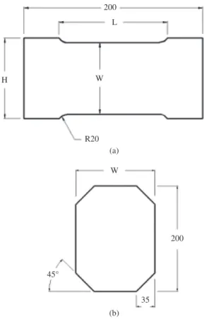
The blank length L is equal to 200 mm which has been taken perpendicular with respect to the rolling direction. The blank width W is equal to 80, 90, 100, 120, 130, 150, 160, 170, 180 and 200 mm so as to cover roughly the drawing (ε1 > 0 and ε2 < 0) and the stretching (ε1 > 0 and
ε2 > 0) regions of the FLC. The geometries and dimensions
of the blank specimens are shown in Figure 2. Carrier or counter-blanks with the same blank material and geometries were also machined so as to prevent the contact between the blank and the flat-punch surfaces and to assure a homogeneous straining. Central holes with diameters equal to 50 and 60 mm were machined in the carrier blanks for the blank specimen widths W = 200 mm and W = 180, 170 and 160 mm, respectively, whereas counter-blanks were cut in two parts (perpendicular to the blank length) for the blank specimen widths W = 80, 90, 100, 110, 130 and 150 mm. All experiments were conducted with a 0.10 mm Teflon sheet between the punch and the carrier-blank, according to the ISO 12004–2:200829 standard. The Marciniak punch tests
were stopped immediately after a drop in the punch load in order to avoid the complete separation of the samples.
2.4.
Strain and roughness measurements
The limit strains are generally determined by carrying out a test up to ductile fracture and, then by analyzing the strain distributions obtained in the vicinity of the fractured zone. The strains are commonly measured using circle or square grids printed or electrochemically etched on the surface of the sheet. The Hecker’s method30 defines
the limit strains as the limiting values between principal surface strains, namely, ε1 and ε2, measured on the necked or fractured sites, and on adjacent circles or squares. The accuracy of strain analysis can also be improved with the help of a digital image correlation (DIC) technique to determine the displacements fields. In the present work, the strain analysis was made using electrochemically etched 2.5 mm square grid with the help of the ASAME target model system31 using both ASTM E 2218 – 0232 and
ISO 12004–2:200829 standards to define the limit strains.
Figure 3 schematically shows the procedure adopted according to the ISO 12004–2:2008 standard to define the limit strains for the specimen blank width W = 120 mm. First, at least three intersections lines nearly perpendicular (within ± 150) to the fracture must be defined to obtain the
The remaining nodes including the ones located on either sides of the border necking area, see Figure 4b, are used to fit the 6th order polynomial. Then, the section limit strains
are obtained by replacing the corresponding peak strain node in the fitted 6th order polynomial equation. Finally,
the major and minor limit strains (ε1, ε2)are defined as the averaged values of the selected sections and the procedure is repeated for each sample width.
Surface roughness measurements were also performed in both as-received and deformed conditions. These measurements were carried out with a portable surface roughness Mitutoyo tester Surftest SJ-301 with a tip radius
of 5 µm using a cut-off length of 2.5 µm and the roughness average (Ra) parameter. Three measurements were made in each Marciniak punch specimen width at two equidistant grid points located on either sides of the fractured regions. The surface roughening was then correlated to the level of the surface effective plastic strain, ε, the initial sheet surface roughness, R0, and the initial grain size, d0, as33:
0 0
R=R +C d ε (3)
In Equation 3, the parameter C is determined from the linear fitting of the plot of R – R0 versus d0ε data. The
accumulated effective plastic strain was calculated assuming
normal plastic anisotropy along with the corresponding Hill’s quadratic34 conjugated effective plastic strain measure
defined under plane-stress conditions as:
1 2
2 2
1 2 1 2
(1 ) 2
1 1 2
r r
r r
+
ε = ε + ε + ε ε +
+ (4)
where: r=(r0+2r45+r90) / 4 is the average normal plastic
anisotropy coefficient while ε1 and ε2 are the principal surface plastic strains determined from the ASAME measurements.
3. Theoretical Analysis
3.1.
Constitutive equations
The constitutive equations are defined within the framework of small strains from the additive decomposition of the total strain-rate tensor, εij, in an elastic part, ij
e
ε , and a plastic part, p
ij ε
, which can be cast in an incremental form as:
p e ij ij ij
dε = ε + εd d (5)
In this work, the elastic strains are neglected in the solution of the localization model adopted to predict the plastic limit strains in sheet metal forming processes. Thus, in order to abridge the notation the superscript p is omitted hereafter. The plastic strain components are defined from the associated plastic flow-rule as:
ij ij
dε = λd ∂f
∂σ (6)
Where: dλ is the plastic multiplier, f is the yield function defined under the assumption of isotropic work-hardening as:
ij
( ) ( , )
f =Fσ - σ ε ε (7)
In Equation 7, F(σij) is a first degree homogeneous stress function which defines the yield surface shape in the stress-space whereas σ is a scalar measure of the effective stress
that defines the yield surface size and can be identified by the measures of effective plastic-strain, ε, and plastic-strain
rate, ε, determined from in the uniaxial tensile test. In this description, the plastic multiplier in Equation 6 can be obtained from the plastic loading condition, that is, f = 0, by firstly applying the Euler’s identity of homogeneous functions of degree n to the yield function given by Equation 7, that is:
( ) ( )
i
i i
i
F F
∂ =
∂ x
x n x
x (8)
and then by calculating the associated plastic-work per unit volume from the equivalent plastic-work principle, namely:
ijd ij d
σ ε = σ ε (9)
Together with the associated flow-rule law, Equation 6, which provides that the plastic multiplier is equal to the effective plastic-strain increment conjugated of the effective stress σ, that is, dλ = εd
The yield function adopted in this work corresponds to the orthotropic plasticity criterion proposed by Ferron et al.35
defined for plane-stress conditions as:
1 2
( , , ) ( , )
f = ϕx x α - σ ε ε (10)
w h e r e : x1 = (σ1 + σ2) / 2 = ( σx x + σy y) / 2 a n d
2 2
2 ( 1 2) 2 ( xx yy) 4 xy
x = σ - σ = σ - σ + σ define the center and the radius of the Mohr’s circle, respectively, as a function of the in-plane principal stress components (σ1,σ2) or else the in-plane orthotropic stress (σxx,σyy,σxy). In Equation 10,
α = (x,1) = (x,2) is the angle of the orientation between the in-plane principal stress directions (1,2) and the in-plane orthotropic symmetry axes (1,2). For numerical implementation purposes, Ferron’s orthotropic plane-stress function is defined as:
1 m 6
2 2 3 2 2 2 2
1 2 1 1 2
2 1 2 1 1 2
m 6 2 2 2
1 2
2
2 2
m 6 2 2 2
1 2
( ) ( )
(1 )
2
( , , ) cos2
(1 ) ( )
b
cos 2
(1 ) ( )
m n n m p q p m
x A x k x x B x k
x x a
x x
k x x
x
k x x
- + - - -
ϕ α = - α
- +
+ α
- +
(11)
In Equation 11, the exponents m, n, p and q are previously known while the material parameters A, B, k, a
and b can be obtained in two steps. Firstly, the parameters (A, B and k) are calculated from the stress-ratios (σb/σ45) and (σb/τ0) between the equibiaxial yield stress, σb, and the uniaxial yield stresses at 450 with respect to the rolling
direction, σ45, and the shear yield stress, τ0, along the rolling direction, respectively, along with the plastic anisotropy coefficient, r45. For steel sheets, the recommended values for the exponents are m = 2, n = 1 or 2, p = 1 or 2 and q = 1 or 235. In particular, a positive value for the parameter k
allows a flattening of the yield surface near plane-strain tension/compression and pure shear stress states. Secondly, the parameters a and b describing the initial in-plane sheet metal anisotropy, can be obtained from the plastic anisotropy coefficients (r0 and r90) or else from the uniaxial yield stresses (σ0,σ45,σ90).
When only uniaxial tension data is available, the parameters defining the yield surface at 450 from the
rolling direction are determined assuming B = 3A and positive k-value. Then, the parameters defining the initial planar material anisotropy, a and b in Equation 11, can be calculated with the r0 and r90 values or else from the stress-ratios (σ45/σ0,σ90/σ0). Also, Hill’s quadratic34
anisotropic yield criterion can be obtained as a particular case of Equation 11 by setting k = 0, m = 2 and n = p = q =1. The yield loci of Ferron’s criterion are plotted in Figure 5 as a function of the angle α in the principal stress space (σ1,σ2) normalized by the equibiaxial yield stress (σb). In this type of representation, g(θ,α) stands for the normalized radius defining a point on the yield locus where θ is the corresponding polar angle which defines the current stress state. The function g(θ,α) is defined as an extension of Drucker’s36 isotropic yield criterion as:
6 6 2 1
2 2
(1 ) ( , ) ( ) 2 sin cos
cos2 sin cos 2
m m m n
p q
k g F a
b
-
-- θ α = θ - θ
θ α + θ α (12)
Where:
2 2 3 2 2 2 2
( ) (cos sin ) cos (cos sin )
Fθ = θ +A θ -k θ θ -B θ (13)
The principal plastic-strain increments are defined with the help of the parametric description, Equation 12, as35:
1
2
d ( , )sin( 4 ) ( , )cos( 4 )
d 2 ( , )
g g
g
ε = θ α π + θ - ′θ α π + θ
ε θ α (14)
2
2
d ( , )cos( 4 ) ( , )sin( 4 )
d 2 ( , )
g g
g
ε = θ α π + θ + ′θ α π + θ
ε θ α (15)
Where: g′( , )θ α ≡ ∂ θ α ∂θg( , ) / . From the metal plasticity incompressibility condition, the plastic anisotropy coefficient defined from an uniaxial tensile test at an angular orientation α with respect to the rolling direction,
i.e., rα = dε2/ dε3 = -dε2/(dε1 + dε2), can be obtained from Equations 14 and 15 as:
4
1 ( , )
1 ( , )
r g
r g
α
α θ=π
∂ θ α =
-+ θ α ∂θ (16)
where: θ = π/4 defines the uniaxial stress state parallel to the in-plane principal stress σ1, as shown by the polar-coordinate description in Figure 5.
On the other hand, the plastic-strain increments in the orthotropic symmetry axes frame (x,y,z) are determined from Equation 6, which depends upon the effective plastic-strain increment and the yield function partial derivatives. The later are obtained by applying the consistency condition,
df = 0, to the Ferron’s yield function defined in the form of Equations 9 and 10, that is:
1 2
1 2
0
dx dx d d
x x
∂ϕ ∂ϕ ∂ϕ
= + + α - σ =
∂ ∂ ∂α
df (17)
and then, by defining the terms dx1, dx2 and dα as a function of the variables (x1,x2) along with the help of the relations sin 2α = σxy/x2 and cos 2α = (σx – σy)/(2x2), which provides:
,xx xx ,yy yy ,xy xy 0
F d F d F d d
= σ + σ + σ - σ =
df (18)
Where: the yield function partial derivatives
,ij ij
F ≡ ∂ ∂σf are given by:
1 2 2
1 sin 2
, cos2
2 2
xx
F
x x x
∂ϕ ∂ϕ α ∂ϕ
= ∂ + α∂ - ∂α
(19)
1 2 2
1 sin 2
, cos2
2 2
yy
F
x x x
∂ϕ ∂ϕ α ∂ϕ
= - α +
∂ ∂ ∂α
(20)
2 2
1 cos2
, 2sin 2 2
xy
F
x x
∂ϕ α ∂ϕ
= α +
∂ ∂α
(21)
While the partial derivative corresponding to the sheet thickness F,zz = –(F, x + F,y) is obtained from the plastic incompressibility condition, that is, dεzz = –(dεx + dεy).
3.2.
Marciniak-Kuczynski model
The localization model developed in this section is an extension of the original theory proposed by Marciniak and Kuczynski3. This model is based upon the existence
of an initial thickness imperfection across the sheet, as depicted in Figure 6, where the superscripts a and b
denote the homogeneous and the defective, respectively. Figure 6 indicates the coordinate systems axes adopted in the present M-K model, where a common frame (O,
n, t, z) is defined by the normal direction n and tangential
t directions to the imperfection and the in-plane normal axis of orthotropy symmetry z. Also, it is assumed that the in-plane orthotropic symmetry axes are coincident to the in-plane principal stress directions in the homogeneous zone a, that is, (xa≡ 1a, ya≡ 2a). In the defective zone, the
orthotropy directions are not coincident with the principal stress directions. This can be taken into account by defining the orthotropic axes (xb, yb) in a corotational frame, which
rotates as a function of the plastic deformation process37,
and is defined by the angle ϕ ≡ (xa, xb) ≡ (ya, yb) shown
in Figure 6. The rotation of the corotational frame axes (xb, yb) with respect to the principal stress directions in the
homogeneous zone a, is defined by37:
b b xx xy b yy (1 ) d d (1 ) + ε
φ = ε
+ ε (22)
where: εbxx and εbyy are the accumulated strains in the
orthotropic symmetry axes and b
xy
dε is the shear-strain increment in the defective zone b.
The M-K geometrical imperfection has an initial angular orientation defined by the angle: Ψ ≡ (xa, n) ≡ (ya, t), see
Figure 6. This angle evolves during the plastic deformation process, which rotation is given by38:
a 1 a 2
(1 d ) tg( ) tg( )
(1 d )
d + ε
ψ + ψ = ψ
+ ε (23)
where: a
1
dε and a 2
dε are the principal strain increments in the homogeneous zone a.
The initial imperfection value is defined by the ratio between the initial thicknesses of the defective zone, t0b,
and homogeneous zone, 0
a
t , as:
0 0 0 b a t f t
= (24)
In this work, the geometrical imperfection is assumed to be dependent on the current sheet roughness R, which is defined by Equation 3, as33:
0 0 0 2 a a t R f t
-= (25)
In Equation 25, the effective plastic strain measure εb
in the geometrical imperfection zone is used in Equation 3 and, thus, the current geometrical imperfection is defined as:
(
)
1/2
0 0 0
0 0 0 2 exp( ) exp exp( ) a b b b b b a zz zz zz
a a a a
zz
t R C d
t t f
t t t
- + ε
ε
= = = ε - ε
ε (26)
The localization problem within the framework of the M-K analysis is based on the equilibrium of forces between the two zones along the normal (n) and tangential (t) directions of the geometrical imperfection, that is:
a b
nn nn
F =F (27)
a b
nt nt
F =F (28)
Which can be written as force per unit width as function of the stress components along the imperfection axes (n,t) and the actual thickness of the two zones, that is:
a a b b
nnt nnt
σ = σ (29)
a a b b
ntt ntt
σ = σ (30)
Also, the geometrical compatibility condition imposes that the strain increments along the tangential direction t
must be the same between the zones a and b, namely,
dε = εatt d btt (31)
The solution of the M-K problem is obtained assuming firstly a given strain-ratio defined in the homogeneous zone between the minor and major in-plane principal strain increments, which is expressed by Ferron’s yield criterion, see Equations 14 and 15, as:
2 1
d ( , )cos( 4 ) ( , )sin( 4 ) ( , )sin( 4 ) ( , )cos( 4 ) d a a a g g g g
ε θ α π + θ + ′θ α π + θ
ρ = =
θ α π + θ - ′θ α π + θ
ε (32)
and, then solving Equation 32 for the angle θ to determine the corresponding stress-state. In the present work, the strain-ratio is varied from the uniaxial tensile stress-state (θUTa = π/ 4) to the equibiaxial straining mode defined by
ρa = 1( a a ES
θ = θ ). Secondly, the homogeneous zone a is loaded incrementally for a fixed strain-ratio (or stress-state) with a small effective-strain increment value (dε =a 10-4). In this way, the stress and strain components in the homogeneous
zone a can be straightforwardly determined. With
Ferron’s orthotropic yield function written in parametric coordinates, see Equation 12, and according to the Figure 6 with the variables x1 σ = σ + σ( 1 2) 2= θ αg( , )cosθ and
2 ( 1 2) 2 ( , )sin
x σ = σ - σ = θ αg θ, one obtains the principal stress components as:
1 ( , )(cos sin )
a ag a a a
σ = σ θ α θ + θ (33)
and
2 ( , )(cos sin )
a ag a a a
σ = σ θ α θ - θ (34)
In Equations 33 and 34 σa is the effective stress measure, which in Ferron’s yield criterion is identified as the equibiaxial yield stress σb. Thus, it is more appropriate to define the stress-strain effective measures in the work-hardening law given by Equation 1 under the equibiaxial tension stress-state. This is achieved noting from Figure 5 that the ratio between the equibiaxial yield stress and the uniaxial tension yield stress at an angular orientation α with respect to the rolling direction is defined by Equations 33 and 34 as σ σ = σ =b/ α bα 2 / [2 (gπ4, )]α , which gives:
1/
3 2 6 /2 1 2
/6
[( 1) ( 1) ] 2 [2 cos2 2 cos 2 2 (1 )
m
m m n p q
b m m
A k B a b
k
-
-α
+ - - - α - α
σ = -
(35)
and then by means of the transformations K=Kα(σbα)Nα+1,
0b 0/ bα
ε = ε σ , ε = ε σ/ bα and ε = ε σ / bα, Equation 1 can
be rewritten as:
0 0
( b )N ( )M
K α α
σ = ε + ε ε ε (36)
Moreover, the stress and strain increments in the geometrical imperfection axes can be obtained from the following transformation equations:
2 2
1cos 2
a a a
nn sen
σ = σ ψ + σ ψ
2 2
1sin 2cos
a a a
tt
σ = σ ψ + σ ψ (37)
2 1
( ) cos
a a a
nt sen
σ = σ - σ ψ ψ
and
2 2
1cos 2
a a a
nn sen
∆ε = ∆ε ψ + ∆ε ψ
2 2
1 2cos
a a a
tt sen
∆ε = ∆ε ψ + ∆ε ψ (38)
2 1
( ) cos
a a a
nt sen
∆ε = ∆ε - ∆ε ψ ψ
The unknowns variables in the weaker zone b, namely,
[ b bnn btt b Tnt]
= ∆ε σ σ σ
X , are then numerically calculated
from the stress and strain states in the homogeneous zone a.
Given that the main governing equations of the M-K problem are defined by two equilibrium forces and one deformation compatibility condition, given by Equations 29-31, an additional relationship is derived from the equivalent principle of plastic-work in the zone b, see Equation 8, so as to obtain a system of four nonlinear equations as proposed by Ganjiani and Assempour39:
1
2
1
b b b b b b
nn nn tt tt nt nt
b b
F =σ ∆ε + σ ∆ε + σ ∆ε
-σ ∆ε (39)
2 1
b tt a tt
F =∆ε
-∆ε (40)
3 1
b nn a nn
F =fσ
-σ (41)
4 1
b nt a nt
F =fσ
-σ (42)
The solution of the system of nonlinear equations
F = [F1F2F3 F4]T is obtained with the help Newton’s
method40, where the initial guess for the solution vector are
set to the values obtained in the homogeneous zone a, that is, X0= ∆ε[ a σann σtta σnta T] . Moreover, a backtracking
algorithm is adopted to assure the convergence of the full Newton’s method which strongly depends on the initial guess39,40. The localized necking criterion is defined when the
ratio between the effective plastic-strain increments in the two zones reaches the condition of an unstable flow, which is given by ∆ε ∆ε ≥b a 10 38. Then, the limit strains are defined
as the corresponding accumulated principal strains in the
homogeneous zone ( , ,
1 , 2 a∗ a∗
ε ε ) by the minimum values of
the major principal strains, 1, a∗
ε , determined as a function of the geometrical imperfection orientation Ψ, which, in turn, is varied between 0 and 90 degrees. Finally, the complete FLC prediction is obtained by varying the strain-ratio in the homogeneous zone ρa between the uniaxial tensile
stress-state and the equibiaxial straining mode.
The effects of non-linear strain-paths are considered assuming bi-linear strain-paths in two stages. In this way, it is possible to analyze the influence of the strain-path upon the forming limits under uniaxial tension, plane-strain tension and equibiaxial stretching pre-straining stages followed by linear proportional strain-paths. The strain components as well the effective plastic strain and the imperfection angular orientation at the beginning of the second stage (2) are initialized with the values determined at the end of the first stage (1):
(1) , (2) ,
, a b a b
a b
ij ij ij
ε = ε + ε (43)
(1) , (2) ,
, a b a b
a b
ε = ε + ε (44)
(2) ,a b (1) ,a b
ψ = ψ (45)
where a given value of the principal strain component is prescribed to the homogeneous zone, (1)1
a
ε , together with
The equations described in this section were coded in Fortran 90 language and all the numerical simulations were performed in an Intel Xeon 5690 3.47 GHz dual-processor workstation with 24 cores and 36 Gb of RAM.
4. Results and Discussion
4.1.
Experimental analysis
4.1.1. Plastic properties
The uniaxial tensile tests were carried out at constant cross-head speeds of 1 and 10 mm/min. The average values determined from 3 tests at each angular orientation (α) of the 0.2% off-set yield stress (σy), the strain-hardening exponent (N), the ultimate tensile strength (σu), the total elongation (∆l) and the Lankford values (r) are listed in Table 2, where the italic values indicate the corresponding standard deviation. The yield stress value increases monotonically between α = 0 and α = 90 degrees, that is, σ90 > σ45 > σ0. As expected, this stress anisotropy is preserved for the ultimate tensile strength values and is also consistent with the angular evolution of the plastic anisotropy coefficient or Lankford values, which decreases monotonically between α = 0 and
α = 900 (r
0 > r45 > r90). The average normal plastic anisotropy
coefficient r=(r0+2r45+r90) / 4 = 2.24 indicates a very good formability level of the analyzed IF hot-dip galvanized steel sheet, mainly for deep-drawing operations.
Table 3 presents the average values of the material parameters fitted according to the work-hardening law defined by Equation 1. The parameters K, ε0 and N in Equation 1 were obtained using a least-squares method from the uniaxial tensile true stress-true plastic strain data at the rolling direction. The IF steel sheet strain-rate sensitivity parameter M was defined as an average value from the fitted average instantaneous strain-rate sensitivity curve, calculated using Equation 2, as a function of the true plastic-strain level, as shown in Figure 7. The predicted true stress-true plastic strain curves computed with the
fitted parameters for the IF hot-dip galvanized steel sheet are in good agreement with the experimental data plotted as a function of the uniaxial tensile test cross-head rate, as shown in Figure 8.
4.1.2. Limit strains andsurface roughness
Figure 9 shows the photograph of the blanks deformed in the Marciniak punch test, where it is possible to observe that the fractured sites are near to the specimen center. Figure 10 presents the contour values of the major and minor principal strains obtained with the ASAME software from the regions
Table 2. IF steel sheet plastic properties determined from uniaxial tensile testing. The italic values indicate the corresponding standard deviation.
α (deg)
σy (MPa)
σu
(MPa) r N ∆1 (%)
0 170.33 296.67 2.65 0.233 42.43
7.37 1.16 0.17 0.003 0.98
45 174.67 301.67 2.11 0.231 42.10
2.31 2.08 0.130 0.001 1.30
90 198.33 303 2.08 0.212 39.93
5.26 7.94 0.08 0.041 5.14
Table 3. IF steel sheet work-hardening parameters fitted from uniaxial tensile data.
K(MPa) N M ε0 ε0(s–1)
576.53 0.309 0.0166 0.0164 3.31 × 10⁻⁴
Figure 7. Fitted and average strain-rate sensitivity parameter M of the hot-dip galvanized IF steel sheet plotted as a function of the uniaxial tensile true plastic-strain.
Figure 8. Experimental and fitted true-stress and true plastic-strain along the rolling direction as a function of the strain-rate.
of interest of each specimen width. The maxima and minima values of the major and minor principal strains (ε1,ε2) varied from (0.87,–0.65) and (0.48, 0.37) for the specimen widths equal to 80 and 200 mm, respectively. It should be noted that none of the probable specimen blank geometries, namely, the widths of 130 and 150 mm, provided the forming limits
close to the plane-strain intercept (FLC0). These unexpected results can be ascribed to the irregular lubrication between the two-piece carrier-blank and the flat-bottomed punch, due to the use of a very thin Teflon sheet (0.1 mm thick), and to the insufficient friction condition between the two-piece carrier-blank and the corresponding specimen blank.
The limit strains determined for the hot-dip galvanized IF steel sheet according to ASTM E 2218-0232 and ISO
12004 –2:200829standards are shown in Figure 11. Firstly,
the limit strains values defined as peer ASTM E 2218-0232
along with the ASAME DIC31 software present a very
large scattering owing to its strong dependence upon the user’s criterion to select the necked and fractured areas at each specimen width. As pointed out, the conducted Marciniak punch tests do not provided points in the FLC near to either sides of the plane-strain intercept due to the uneven friction conditions. The software trend forming limit curves at necking and fracture conditions are also shown in Figure 11a, providing a forecast for the plane-strain intercept FLC0. Conversely, the limit strains defined according to ISO 12004 –2:200829, see Figure 11b, clearly show the couple of
strains determined for each specimen thanks to the rejection and fitting procedures to delimitate the border of the necking zone from either sides of the peak strain. It should be noted that the fracture limit strains were obtained from the reconstruction of the grid pattern performed with the ASAME software and as the peak strain using the ASTM E 2218-0232 and ISO 12004 –2:200829 standards, respectively.
The IF hot-dip galvanized steel sheet presents a very good formability level in the deep-drawing range thanks to its elevated plastic anisotropy coefficients.
Due to the lack of the experimental limit strains close to the plane-strain intercept, the empirical formula proposed by Keeler and Brazier41 is adopted here to forecast the
engineering FLC0 value:
(23.3 14.13 )
(%)
0.21
0N
FLC
=
+
t
(46)Where: t is the sheet thickness expressed in mm
a n d N=(N0+2N45+N90) / 4=0.227 i s t h e a v e r a g e strain-hardening exponent calculated from the uniaxial tensile data listed in Table 2. Henceforth, the corresponding true plane-strain intercept predicted value, εPS∗ =0.311, will be
adopted together with the limit strains determined according to the ISO 12004 –2:200829 for comparison purposes with the
theoretical predictions of the present M-K model.
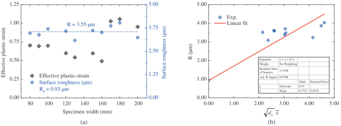
Figure 12a correlates the resulting effective plastic-strains calculated with Equation 4 and the measured average roughness (Ra) values as a function of the specimen width. The average initial roughness of the IF hot-dip galvanized
Figure 11. Limit strains of the hot-dip galvanized IF steel sheet determined according to the (a) ASTM E 2218 – 0232 and (b) ISO 12004–2:200829 standards.
steel sheet is R0 = 0.93 µm and changed to an average value of R=3.55 µm due to the in-plane plastic straining. Figure 12b shows the plot of the R – R0 versus d0ε data
and the linear fitting according to the Equation 3, from which the resulting C parameter is equal to 0.773 µm1/2.
4.2.
Theoretical predictions
4.2.1. Validation of the M-K model
In order to validate the M-K model developed in the present work, see Section 3.2, we first present the theoretical predictions for linear and bi-linear strain-paths assuming material models as a function of the plastic anisotropy coefficient. Then, the predictions determined with Hill’s quadratic34 and Ferron’s35 yield criteria are compared to
the experimental data obtained from linear and bi-linear strain-paths for an AISI-1012 steel sheet with a nominal thickness of 2.5 mm[42]. Table 4 lists the sheet material
plastic properties adopted in all the theoretical predictions discussed in the present section. From Equation 25, the initial value of the geometrical imperfection f0 for the AISI-1012 steel sheet is equal to 0.995. Figure 13a presents linear strain-paths predictions determined as a function of the value of the plastic anisotropy coefficient at 450 with
respect to the rolling direction. Three material models have been defined assuming r45 equal to 0.5, 1.0 and 2.5 together with r0 = r90=1.0, respectively. The present material parameter combinations have already been investigated by Barata da Rocha et al.38 and were adopted here to verify
the consistence of the present M-K model predictions. For the planar-anisotropic materials, the numerical simulations were performed with Hill’s quadratic yield criterion34
while the von Mises yield criterion was adopted for the isotropic case. As expected, the same limit strains values are predicted under the uniaxial tensile strain-mode since all the adopted materials models have the same plastic anisotropy coefficient in the rolling direction and, thus,
0/ (1 0) 0.5 a
r r
ρ = - + = - . Conversely, in the biaxial stretching domain the limit strains are strongly affected when the plastic anisotropy coefficient r45 is > 1.0 whereas the same FLC’s are obtained for the isotropic (r45 = 1.0) and r45 < 1.0 cases. Moreover, it should be noted that these material parameters provide equal in-plane principal stress-ratio in the equibiaxial stretching stress-state condition, namely,
2 1 1.0
β = σ σ = . These differences are attributed to the geometrical imperfection orientation Ψ which minimizes the computed limit strains, as shown in Figure 13b in the plot of the corresponding critical major principal strains,
, 1a∗
ε , as a function of the orientation Ψ. The minimum limit strain for the r45 > 1,0 case is obtained for Ψ ≅ 45 degrees whereas ther45 < 1.0 material has minima coincident with isotropic reference case for Ψ = 0 and 90 degrees. As pointed out by Barata da Rocha et al.38, the original assumption of
normality of the geometrical imperfection with respect to major in-plane principal stress19 is too restrictive since
it would provide a unique limit strain in the equibiaxial stretching condition independently of the r45 value.
Figure 14 compares the theoretical predictions for an isotropic (von Mises) material determined from linear strain-paths and bi-linear strain-paths after a pre-straining level of 15% under uniaxial tension (UT), plane-strain tension (PS) and equibiaxial straining (ES) conditions, respectively. In comparison to the linear strain-paths predicted values, it is possible to observe that the limit strains increase in the biaxial strain domain after the same amount of pre-strain under UT and PS conditions. In the deep-drawing range, that is, for negative minor principal strains, the resulting limit strains from the second deformation stage decreased after a UT pre-straining and are improved after a pre-straining under PS condition. Conversely, the influence of the ES pre-straining is more pronounced given that a remarkable decrease of the limit strains in biaxial strain range and an increase in the Table 4. AISI-1012 steel sheet material properties42.
K(MPa) N M ε0 d0 (µm)
238 0.35 0.01 0.01 25
R (µm) C (µm1/2) r
0 r45 r90
6.5 0.104 1.40 1.05 1.35
negative minor principal strain domain. Except for the PS case, the plane-strain intercept of the FLC moved towards the pre-straining mode direction, namely, shifted-up after the UT pre-straining and drastically decreased after the ES pre-straining stage. It should be pointed out that the above
bi-linear strain-path calculations were performed without unloading between the first and second stages.
Figures 15 and 16 compare the predicted FLCs with the experimental results determined for an AISI-1012 steel sheet42 from linear and bi-linear strain paths, respectively.
The parameters adopted in Ferron’s plasticity yield criterion were m = n = 2, p = q = 1 with k = 0.15. The parameters
a and b which describe the in-plane sheet metal plastic anisotropy in Ferron’s criterion, see Equation 11, were determined from the plastic anisotropic coefficients r0 and r90. The linear strain-path predictions obtained with both Hill’s and Ferron’s yield criteria are in good agreement with the experimental data near the plane-strain intercept of the AISI-1012 FLC whereas either anisotropic yield criteria underpredict the limits strains for larger values of the in-plane negative minor principal strain, as shown in Figure 15. In the biaxial stretching domain, a better approximation is achieved with Ferron’s anisotropic yield criterion predictions. This is attributed to the flattening of Ferron’s yield surface near to plane-strain tension/compression and pure shear stresses states, thanks to a positive k-value in Equation 11, providing a smaller ratio between the major principal plane-strain yield stress, σPS1, and the equibiaxial yield stress, σb, namely, the material parameter P = σPS1/σb
introduced by Barlat8, in comparison with Hill’s quadratic
plane-stress yield locus. Figure 16a compares the theoretical predictions with the experimental AISI-1012 limit strains obtained after 10% of pre-strain in uniaxial tension. As for the linear strain-path, either yield criteria provided a good forecast near to the shifted plane-strain intercept. However, the corresponding theoretical predictions overestimate and underestimate the experimental data for the levels of the minor principal strain –0.20 ≤ ε2 ≤ –0.10 and –0.40 ≤ ε2 ≤ –0.30, respectively. Figure 16b shows that either yield criteria predictions underestimate the experimental limit strains after 8% of pre-strain in equibiaxial tension.
Recently, Nurcheshmeh and Green43 developed a M-K
model based upon a mixed isotropic-nonlinear kinematic hardening along with Hill’s quadratic yield description obtaining improved predictions for the cited AISI-1012 steel sheet limit strains under bi-linear strain-paths.
Figure 14. Theoretical predictions determined for an isotropic material from bi-linear strain-paths as a function of pre-strain mode: UT - Uniaxial Tension, PS - Plane-Strain and ES - Equibiaxial Straining.
Figure 15. Comparison between the experimental linear strain-path forming limits of a low carbon steel sheet42 and theoretical predictions obtained by the M-K model with Hill’s quadratic34 and Ferron’s35 anisotropic yield criteria.
quadratic and Ferron’s criteria, parameters a and b in Equation 11, were determined from the uniaxial tensile data assuming firstly B = 3A and, then, by exchanging the r0 and r90 experimental values. Also, the work-hardening law was transformed according to the Equation 36 by setting α = π/2 in Equation 35 since the effective stress measure in Ferron’s orthotropic yield criterion is identified by the equibiaxial yield stress (σ1 = σ2 = σb). Both yield criteria descriptions provided a very good agreement with the experimental limit strains located in the drawing range and a good match with the empirical FLC0. This can be attributed to the description of the geometrical imperfection parameter of the M-K model based upon the experimental evolution of the surface roughness as a function of the mean initial grain size and the effective plastic-strain. On the other hand, only Ferron’s orthotropic plasticity yield criterion provided a good prediction of the experimental limit strains in the biaxial stretching range. This is accredited to the yield surface shape in the region of interest, namely, the existence of a flattening in Ferron’s yield locus between the equibiaxial and plane-strain tension stress-states, which, in turn, provide a decrease in the stress-ratio P = σPS1/σb in comparison to the Hill’s quadratic yield surface. Thus, for a given strain-path ρ = ε2/ε1 or else a stress-ratio β = σ2/σ1, the strain localization in the imperfection zone of the M-K model is favored as the parameter P decreases. This yield surface shape effect is better explained in Figure 18, where the limit strains predictions of the adopted anisotropic yield criteria are plotted in the biaxial stretching range with the computed history strain-paths in both homogeneous (circle-dot lines) and imperfection (dashed lines) zones of the M-K localization model. First, one can observe the strain-path changes towards a plane-strain state in the imperfection zone and, then, the earlier plastic localization with Ferron’s yield criterion.
4.2.2. Predicted FLC
Figure 17 compares the experimental limit strains determined for the IF hot-dip galvanized steel sheet with the theoretical predictions of the M-K model based upon the Hill’s quadratic34 and Ferron’s35 yield criteria. From
Equation 25 with the initial average roughness value of 0.93 mµ, the initial value of the geometrical imperfection of the M-K model f0 is equal to 0.997. The parameters adopted in Ferron’s orthotropic plasticity yield criterion were m = n = p = q = 2 and k = 0.2. It should be recalled that the experimental limit strains are defined according to the ISO 12004 –2:200829 as well as that the plane-strain
intercept value has been predicted according to Equation 46. Given that the Marciniak punch tests were performed with the specimen blank length perpendicular to the rolling direction, the material anisotropic parameters of Hill’s
Figure 17. Comparison between the experimental linear strain-path forming limits of a hot-dip galvanized interstitial-free steel sheet and theoretical predictions obtained by the M-K model with Hill’s quadrati34 and Ferron’s35 anisotropic yield criteria.
the assumption of isotropic work-hardening forecasted only the experimental trends of the low carbon steel FLCs determined from bi-linear strain-paths after uniaxial and biaxial tension pre-straining. The M-K geometrical imperfection parameter was defined more properly from the experimental correlation of the surface roughness changes described as a function of the accumulated effective plastic strain and the mean grain size of the investigated hot-dip galvanized interstitial-free steel sheet. In the deep-drawing range, both Hill’s quadratic and Ferron’s yield criteria provided a good agreement with the limit strains of the hot-dip galvanized interstitial-free steel sheet. Only Ferron’s description forecasted the experimental data in the biaxial stretching domain owing to the effect of the yield surface flattening near to the plane-strain tension stress-state.
Acknowledgements
The authors acknowledge CNPq and FAPERJ for the research grants which supported this work and CSN for providing the sheet material and facilities to perform the experimental testing. MCSF acknowledges CAPES for the PhD. scholarship.
5. Conclusions
In the present work, experimental and theoretical analyses of the limit strains of a hot-dip galvanized interstitial-free steel sheet were performed with the help of the Marciniak punch test technique and based on the M-K localization model, respectively.
The investigated hot-dip galvanized interstitial-free steel sheet presented a very good formability level, which is suitable for exposed parts in which an extra deep-drawing quality is often required. However, the adopted experimental procedure to conduct the FLC tests revealed to be too susceptible to the lubrication conditions between the flat-bottomed punch and the carrier-blank. Besides, the limit strains defined as per ISO 12004-2:2008 has proven to be more consistent vis-à-vis the ASTM E 2218 – 02 standard procedures. The proposed M-K model based upon both Hill’s quadratic and Ferron’s anisotropic yield criteria was first validated by means of comparisons with available data of a low carbon steel (AISI 1012) for linear and bi-linear strain-paths. Under linear strain-paths, reasonable agreement was obtained from Ferron’s orthotropic yield criterion predictions. Conversely, either adopted yield criteria under
References
1. Keeler SP. Determination of the forming limits in automotive stamping. Sheet Metal Industries. 1965; 461:683-691.
2. Goodwin GM. Application of the strain analysis to sheet metal forming in the press shop. La Metallurgia Italiana. 1968; 8:767-774.
3. Marciniak Z and Kuczynski K. Limit strains in the processes of stretch-forming sheet metal. International Journal of Mechanical Sciences. 1967; 9:609-620. http://dx.doi. org/10.1016/0020-7403(67)90066-5
4. Hutchinson JW and Neale KW. Sheet necking-III. Strain-rate effects. In: Koistinen DP and Wang NM, editors. Mechanics of Sheet-Metal Forming. New York: Plenum Press; 1978. p. 269-285. http://dx.doi.org/10.1007/978-1-4613-2880-3_11
5. Neale KW and Chater E. Limit strain predictions for strain-rate sensitive anisotropic sheets. International Journal of Mechanical Sciences. 1980; 22:563-574. http://dx.doi. org/10.1016/0020-7403(80)90018-1
6. Sowerby R and Duncan JL. Failure in sheet metal in biaxial tension. International Journal of Mechanical Sciences. 1971; 13:217-229. http://dx.doi.org/10.1016/0020-7403(71)90004-X
7. Ferron G and Mliha-Touati M. Determination of the forming limits in planar-isotropic and temperature-sensitive sheet metals. International Journal of Mechanical Sciences. 1985; 27:121-133. http://dx.doi.org/10.1016/0020-7403(85)90053-0
8. Barlat F. Crystallographic texture, anisotropic yield surface and forming limits of sheet metals. Materials Science Engineering. 1987; 91:55-72. http://dx.doi.org/10.1016/0025-5416(87)90283-7
9. Cao J, Yao H, Karafillis A and Boyce MC. Prediction of localized thinning using a general anisotropic yield criterion, International Journal of Plasticity. 2000; 16:1105-1129. http:// dx.doi.org/10.1016/S0749-6419(99)00091-1
10. Wu PD, Jain M, Savoie J, MacEven SR, Tugcu P and Neale KW. Evaluation of anisotropic yield functions for aluminum
sheets. International Journal of Plasticity. 2003; 19:121-138. http://dx.doi.org/10.1016/S0749-6419(01)00033-X
11. Barlat F, Lege DJ and Brem JC. A six-component yield function for anisotropic materials. International Journal of Plasticity. 1991; 7:693-712. http://dx.doi.org/10.1016/0749-6419(91)90052-Z
12. Karafillis A and Boyce MC. A general anisotropic yield criterion using bounds and transformation weighting tensor. Journal of the Mechanics and Physics of Solids. 1993; 41:1859-1886. http://dx.doi.org/10.1016/0022-5096(93)90073-O
13. Barlat F, Maeda Y, Chung K, Yanagawa M, Brem JC, Hayashida Y et al. Yield function for aluminum alloy sheets. Journal of the Mechanics and Physics of Solids. 1997; 45:1727-1763. http:// dx.doi.org/10.1016/S0022-5096(97)00034-3
14. Alwood JM and Shouler DR. Generalised forming limit diagrams showing increased forming limits with non-planar stress states. International Journal of Plasticity. 2009; 25:1207-1230. http://dx.doi.org/10.1016/j.ijplas.2008.11.001
15. Eyckens P, Van Bael A and Van Houtte P. Marciniak-Kuczysnki type modelling of the effect of through-thickness shear on the forming limits of sheet metal. International Journal of Plasticity. 2009; 25:2249-2268. http://dx.doi.org/10.1016/j. ijplas.2009.02.002
16. Eyckens P, Van Bael A and Van Houtte P. An extended Marciniak-Kuczysnki model for anisotropic sheet subjected to monotonic strain paths with through-thickness shear. International Journal of Plasticity. 2011; 27:1577-1597. http:// dx.doi.org/10.1016/j.ijplas.2011.03.008
17. Assempour A, Nejadkhaki HK and Hashemi R. Forming limit diagrams with the existence of through-thickness normal stress. Computational Materials Sciences. 2010; 48:504-508. http:// dx.doi.org/10.1016/j.commatsci.2010.02.013
18. Nurcheshmeh M and Green DE. Influence of out-of-plane compression stress on limit strains in sheet metals. International Journal of Material Forming. 2011; 5(3):1-15.
32. American Society for Testing and Materials – ASTM. E 2218:02: Standard Test Method for Determining Forming Limit Curves. ASTM International, 100 Barr Harbor Drive, PO Box C700, West Conshohocken, PA 19428-2959, United States.
33. Gronostajski JZ and Zimniak Z. The effect of changing of heterogeneity with strain on the forming limit diagram. Journal of Materials Processing Technology. 1992; 34:457-464. http:// dx.doi.org/10.1016/0924-0136(92)90141-E
34. Hill R. A Theory of the yielding and plastic flow of anisotropic metals. Proceedings of the Royal Society of London. 1948; A193:281-297.
35. Ferron G, Makkouk R and Morreale J. A parametric description of orthotropic plasticity in metal sheets. International Journal of Plasticity. 1994; 10:51-63. http://dx.doi.org/10.1016/0749-6419(94)90008-6
36. Drucker DC. Relation of experiments to mathematical theories of plasticity. Journal of Applied Mechanics, Transactions of the ASME. 1949; 16:349-357.
37. Arrieux R and Boivin M. Détermination théorique du diagramme des contraintes limites de formage. Application aux matériaux anisotropes. European Journal of Mechanical Engineering. 1992; 37:89-96.
38. Barata da Rocha A, Barlat F and Jalinier JM. Prediction of the forming limit diagrams of anisotropic sheets in linear and non-linear loading. Materials Science Engineering. 1985; 68:151-164. http://dx.doi.org/10.1016/0025-5416(85)90404-5
39. Ganjiani M and Assempour A. Implementation of a robust algorithm for prediction of forming limit diagrams. Journal of Materials Engineering and Performance. 2008; 17:1-6. http:// dx.doi.org/10.1007/s11665-007-9121-4
40. Press WH, Teukolsky SA, Vetterling WT and Flannery BP. Numerical Recipes in Fortran 77. 2nd ed. Cambridge University Press, 1996. chap. 9, v. 1.
41. Keeler SP and Brazier WG. Relationship between laboratory material characterization and press shop formability. Microalloying. 1977; 75:517-530.
42. Molaei B. Strain path effects on sheet metal formability. [Thesis]. Iran: Amirkabir University of Technology, 1999.
43. Nurcheshmeh M and Green DE. Prediction of sheet forming limits with Marciniak and Kuczynski analysis using combined isotropic–nonlinear kinematic hardening. International Journal of Mechanical Sciences. 2011; 53:145-153. http://dx.doi. org/10.1016/j.ijmecsci.2010.12.004
for sheet metal in tension. International Journal of Mechanical Sciences. 1973; 15:789-805. http://dx.doi.org/10.1016/0020-7403(73)90068-4
20. Chan KS. Marciniak-Kuczynski approach for calculating forming limit diagrams. In: Wagoner RH, Chan KS and Keeler SP, editors. Forming Limit Diagrams: Concepts, Methods and Applications. TMS; 1989. p. 73-110. PMid:2917344. 21. Barlat F. Forming limit diagrams – Predictions based on some
microstructural aspects of materials. In: Wagoner RH, Chan KS and Keeler SP, editors. Forming Limit Diagrams: Concepts, Methods and Applications. TMS; 1989. p. 275-301. 22. Chu CC and Needleman A. Void nucleation effects
in biaxially stretched sheets. Journal of Engineering Materials and Technology. 1980; 102:249-256. http://dx.doi. org/10.1115/1.3224807
23. Tvergaard V. Effect of yield surface curvature and void nucleation on plastic flow localization. Journal of the Mechanics and Physics of Solids. 1987; 35:43-60. http://dx.doi. org/10.1016/0022-5096(87)90027-5
24. Gänser HP, Werner EA and Fischer FD. Forming limit diagrams: a micromechanical approach. International Journal of Mechanical Sciences. 2000; 42:2041-2054. http://dx.doi. org/10.1016/S0020-7403(99)00057-0
25. Kristensson O. Numerically produced forming limit diagrams for metal sheets with voids considering micromechanical effects. European Journal of Mechanics – A/Solids. 2006; 25:13-23. http://dx.doi.org/10.1016/j.euromechsol.2005.05.007 26. Wu PD, MacEwen SR, Lloyd DJ and Neale KW. A mesoscopic
approach for predicting sheet metal formability. Modeling and Simulation in Materials Science and Engineering. 2004; 12:511-27. http://dx.doi.org/10.1088/0965-0393/12/3/011
27. Associação Brasileira de Normas Técnicas – ABNT. NBR ISO 6892:2002: Metallic materials - Tensile testing at ambient temperature. ABNT; 2002.
28. Nakazima K, Kikuma T and Hasuka T. Study on the formability of steel sheets. Yawata Technical Report. 1968; 284:140-141, 1968.
29. International Organization for Standardization – ISO. 12004-2:2008 (E): Metallic materials – Sheet and strip – Determination of forming limit curves – Part 2: determination of forming limit curves in laboratory. Geneva: ISO; 2008.
30. Hecker SS. Simple Technique for Determining Forming Limit Curves. Sheet Metal Industries. 1975; 52:671-676.