HUB LOCATION UNDER HUB CONGESTION AND DEMAND UNCERTAINTY: THE BRAZILIAN CASE STUDY
Gilberto de Miranda Junior
1*, Ricardo Saraiva de Camargo
2,
Luiz Ricardo Pinto
3, Samuel Vieira Conceic¸˜ao
4and Ricardo Poley Martins Ferreira
5Received February 1, 2010 / Accepted March 17, 2011
ABSTRACT.In this work, a mixed integer nonlinear programming model combining direct service links, demand uncertainty and congestion effects is proposed. This model is efficiently solved by Generalized Benders Decomposition, for instances of moderate sizes and reasonable number of scenarios. The deployed algorithms are further used for re-designing the Brazilian air transportation network, enabling the analysis of future demand scenarios and providing decision support about the optimal investment policy for Brazil.
Keywords: hub-and-spoke networks, Benders Decomposition, large scale optimization, mixed integer non-linear programming, demand uncertainty.
1 INTRODUCTION
In the last few years, the Brazilian air transportation network has gone through several operational breakdowns. The apparent reason is the lack of capacity or infra-structure on the main airports of the system. But a closer look of the network reveals that the total installed capacity is much larger than the total traffic volume to be handled, indicating that the network seems to operate in a sub-optimal way. As a consequence, the network performance has been severely compromised, reducing the opportunity of the involved logistic operators for attaining the economies of scale that lead to sustainable revenues.
*Corresponding author
1Departamento de Engenharia de Produc¸˜ao, Universidade Federal de Minas Gerais, Belo Horizonte, MG, Brasil. E-mail: [email protected]
2Departamento de Engenharia de Produc¸˜ao, Universidade Federal de Minas Gerais, Belo Horizonte, MG, Brasil. E-mail: [email protected]
3Departamento de Engenharia de Produc¸˜ao, Universidade Federal de Minas Gerais, Belo Horizonte, MG, Brasil. E-mail: [email protected]
4Departamento de Engenharia de Produc¸˜ao, Universidade Federal de Minas Gerais, Belo Horizonte, MG, Brasil. E-mail: [email protected]
In order to provide the necessary operational efficiency to this system, as well as to define opti-mal investment policies considering the system expansion and future demand sceneries, a mixed integer non-linear programming formulation is proposed. This model aims to redesign the cur-rent network, optimizing the use of the installed capacity and balancing the flows through the network. Here, the underlying structure adopted for the Brazilian air transportation network is a customized hub-and-spoke topology. The desired effect is eventually to deactivate some of the current network hubs while activating several others to handle the additional third party traffic.
Hub-and-spoke systems have been largely employed in the telecommunication and transportation areas (see [18, 43, 4, 42, 14]). This class of systems arises when commodities (passenger, cargo parcels, telecommunication packets) of a set of origins must be sent to a set of destinations. Instead of establishing a direct connection for each origin-destination pair, facilities that serve as switching, transshipment, sorting and distribution nodes, designated as hubs, are used as the only valid intermediate points in a path from an origin to a destination. Flows from different origins are gathered at these hub facilities prior to be routed to an intermediate hub or to be delivered to their final destinations.
The employment of these hub facilities and the routing of consolidated flows through inter-hub links allow the centralization of commodity handling and the transportation cost per unit of flow to be less expensive than directly shipping via a non-hub network structure. In other words, the hub networks take advantage of scale economies on inter-hub connections [58, 59].
Usually, the main concerns of hub network design are the location of hub facilities and the al-location of non-hub nodes to hubs at the least expensive network structure, accounting for that the installation and the transportation costs. This is done by selecting node candidates as hubs and assigning origin and destination nodes to these hubs, given the flow volumes between each origin-destination node pair, the installation costs of hubs and the transportation costs between nodes of the network. While hubs are in general fully connected among them, non-hub nodes can be single allocated, meaning that a non-hub can be assigned to exactly one hub only; and mul-tiple allocated, meaning that a non-hub can be connected to more than one hub of the network. Alternative configurations can be considered in order to ensure the application of a specific pro-tocol [62]. For further basic notions, different considerations and formulations of hub networks see the comprehensive surveys of Campbell [12, 13] and of Campbellet al.[14] and of Alumur & Kara [2].
The minimization of the installation and transportation costs approach generates solutions that tend to overload a small number of hubs, forcing the congestion effects into consideration. The hub literature has been dealing with the congestion cost effects on hub networks implicitly, when these effects are represented by constraints, and explicitly, when the congestion costs are expres-sed on the objective function.
A great variety of researchers has tackled the congestion effects restricting the amount of flow transiting through a hub by means of capacity constraints. Aykin [3] has devised a lagrangian relaxation approach, while Ernst & Krishnamoorthy [27] have used simulated annealing and random descent methods. Eberyet al. [23] have imposed capacities only on incoming flows. They have developed a branch-and-bound based on a shortest path heuristic. Solutions obtained by their method may have flows from a hub to itself routed via another hub as explained by Campbellet al.[14]. Campbellet al.[17, 15, 16] have proposed the hub arc location problem, in which the hub network is seen as a three-layered network. The bottom one has the origin nodes of the demand, the middle layer has the hub nodes, and the top one has the destination nodes of the demand.
Yaman & Carello [72] have addressed the problem of solving single allocation hub location problems with modular link capacities. They have proposed a non-linear formulation where the size of inter-hub connections are treated as stepwise, instead of the linear approach proposed by Labb´eet al. [44] to the quadratic capacitated hub location problem with single assignment. In order to accomplish that, capacity restrictions have been imposed on the amount of traffic flowing through the hubs rather than only considering the incoming traffic. The problem has been solved by means of an branch-and-cut algorithm based on a linearization with an exponential number of constraints and a two-level local search method. Both methods have been then combined in a heuristic concentration (see [68, 67]) scheme. Mar´ın [54] also has addressed the capacitated multiple allocation hub location problems, but assumed that the flow between a given origin-destination pair can be split into several routes.
Another interesting work is the one presented by Kara & Tansel [41]. They have modeled the transient times at hubs in addition to the travel times, having as objective function the minimi-zation of the latest-arrival times, and consequently, the excessive delays at the hubs. Yamanet al.[73] have presented a similar formulation for a Turkish cargo delivery system where transient times have been taken into account as well as journey times.
A work that stands out is the one of Marianov & Serra [53]. They have modeled the hub network as an M/D/c queuing network, proposing capacity constraints based on the probability of waiting customers in the system. Due to the computational complexity of these constraints, they have linearized them and then solved the resulting model by a tabu search algorithm. A similar work has been proposed by Rodriguezet al.[65], but a simulated annealing algorithm has been used.
Modeling congestion through capacity constraint on the flows does not mimic the exponential nature of the congestion effects. Elhedhli & Hu [24] have been the first ones to consider the costs of the congestion effects explicitly on the objective function. Using a convex cost function that increases exponentially as more flows go through the hubs, they have proposed a non-linear model to a single assignment hub location problem. The congestion convex cost function is a power-law function of airport usage relative to its capacity and it has been widely used to estimate delay costs [35]. They have linearized their model and then solved it using lagrangian relaxation.
On the other hand, stochastic location problems where demand uncertainties are taken into ac-count have been addressed by G. Albareda-Sambolaet al. [1], Hochreiter & Pflug [40], Snyder et al.[70], Gabor & Van Ommeren [31], Snyder & Daskin [69], Laporteet al.[46], Louveaux & Peeters [48], Laporteet al.[45] and Franc¸a & Luna [28]. In all these works, it is established that stochastic modeling provides a superior design by considering uncertainty in important parame-ters. When dealing with HS network design, it is interesting to consider the demand uncertainty, since, according to Camargoet al. [10], the impact of demand components in the optimal HS network under congestion is considerable. Another interesting conclusion of Camargoet al.[10] is that under huge congestion, the marginal utility of installing a new hub in the HS network is reduced. This counter-intuitive effect is due to the HS classical protocol – if a given demand is considerably high, it is not interesting to have this link on the HS network, since it will always imply in high congestion. It is clear that if a given node is overloaded with his own demand, it is unable to handle third party traffic. It is also uninteresting to route such high flows trough a hub, under penalty of severely impact the hub performance. A further step could be the allowance of direct routes between non hub nodes, where no economy of scale is observed but no congestion either.
In this paper, we explore further the congestion effects written as a convex cost function similarly to [24], but addressing the multiple allocation hub location problem, considering also effects of demand uncertainty combined with direct service links. We propose a non-linear mixed integer programming problem based on a classical formulation [37] due to its linear programming bound quality when compared to others [12, 25, 26, 61]. In our formulation the number of hubs on a route is limited to two, even if there is a route with a lower cost using more than two hubs.
Although, one of the main strategies to handle non-linear problems is to linearize them, we have developed a Generalized Benders Decomposition (GBD) [33] to cope with our non-linear mixed integer program. The problem is decomposed in two smaller problems: at a higher level, named as master problem (MP), the location decisions are made; while at an inferior level, known as subproblem (SP), the flow balance and the congestion are handled. The MP is an integer programming problem, while the SP is a non linear convex transportation problem. Using our approach, we have been able to solve some large problems of the CAB and AP standard data sets to optimality. We have also used the deployed algorithm to deal with a real hub location case, studying the Brazilian air transportation network.
pro-blem and it is also demonstrated how the subpropro-blems can be optimally solved. Computational experiments and conclusion remarks are presented in Section 4 and 5, respectively.
2 MODEL FORMULATION
In this section the our model formulation efforts are presented. The basic components of the model are the following sets: letNbe the set of node locations that exchange traffic and letHbe the set of node candidates to become hubs,H ⊆N. For any pair of nodesiandj(i,j ∈N), we havewi j, the flow from origini to destinationjthat is routed through either one or two installed
hubs. Usually, we havewi j 6=wji.
Further, let fk be the fixed cost of installing a hub at nodek ∈ H and letci j kmbe the
transpor-tation cost per unit of flow from nodei to j routed via hubskandm(i,j ∈ Nandk,m ∈ H). This transportation cost is the composition of three cost segments: ci j km =ci k+αckm+cm j,
where ci k and cm j are the standard transportation cost per unit from locationi (j) to hubk
(m), andαckmis the discounted transportation cost between hubskandm. The discount factor
0≤α≤ 1 represents the scale economies on the inter-hub connection. If only one hub is used in a given route, we havek=mand no discount factor is applied.
The following decision variables are defined:
yk= (
1, if hub k∈ His installed; 0, otherwise.
xi j km ≥0 is the flow from origini to destination j (i,j ∈ N) that is routed through hubs
kandm(k,m∈ H) in that order.
In order to start the development of the congested version of the uncapacitated multiple allocation hub location problem (UMAHLP), the formulation due to Hamacheret al.[37] is stated as:
minX
k
fk yk+ X
i X
j X
k X
m
ci j km xi j km (1)
s. t.:
X
k X
m
xi j km =wi j ∀i,j ∈ N (2)
X
m
xi j km+ X
m6=k
xi j mk ≤wi j yk ∀i,j ∈ N, k∈ H (3)
xi j km ≥0 ∀i,j ∈ N, k,m∈H (4)
yk ∈ {0,1} ∀k∈ K (5)
In Camargoet al. [11] the above formulation has been used to solve instances up to 200 nodes with the aid of Benders decomposition. In this sense, formulation (1)-(5) is adopted as a basis to develop a congested approach to hub location due to its nice theoretical properties and good structure. Hamacheret al. [37] have demonstrated that constraints (3) are facet defining. In addition, for a fixed hub structure, the remaining formulation is fully decomposable for each i−jpair. In spite of this, O’Kelly & Brian [60] have shown that having the same discount factor αfor all the inter-hub connections may be unrealistic. Optimal solutions where large discounts are given on links having small flows can be generated in this way. Overcoming this drawback, a hub location formulation with flow-dependant economies of scale can be addressed, as proposed by Camargoet al.[9].
In order to allow the use of direct service links, is necessary to add a new set of variables:
θi j ≥0 is the amount of flow transported through a direct connection for pairi−j.
It is also necessary to modify constraints (2) to include the direct paths, producing:
θi j+ X
k X
m
xi j km=wi j ∀i,j ∈ N (6)
Implying to rewrite the objective function as:
minX
k
fk yk+ X
i X
j X
k X
m
ci j km xi j km+ X
i X
i
ci j θi j (7)
Moreover, Mar´ınet al.[55] have shown how formulation (1)-(5) can allow optimal solutions with routes having more than two hubs when the triangular inequalities are not satisfied. Instead of using the constraints derived by Mar´ın to deal with those possible unfeasible paths, the following additional constraints are preferable in a decomposition framework, since they preserve thei−j pair decomposition:
xi ji j ≥wi j (yi +yj−1) ∀i,j ∈ N (8)
X
k6=j
xi ji k ≥wi j (yi −yj) ∀i,j ∈ N (9)
X
k6=i
xi j k j ≥wi j (yj−yi) ∀i,j ∈ N (10)
Constraints (8) make sure that the flowwi j goes through routei−j−i−jwheniandjare hubs.
gk ≥0 is the total flow which goes through hubk∈H.
Further, a set of additional coupling constraints have to be added in order to amount the total flow in a given hub:
X i X j X m
xi j km+ X
i X
j X
m6=k
xi j mk =gk ∀k∈ H (11)
A congestion cost functionτk(gk)is assumed as given for each installed hub k ∈ H. This
function is considered increasing on[0,+∞), proper convex and smooth. It is responsible for distributing the flow load along each installed hub, thus reducing the overall congestion expressed in monetary values. The congestion cost function used is a power law whereτk = e gkb, and
eandb are positive constants,b ≥ 1. This class of functions has been already used by [24] to the single allocation case and by [10] in his recent work. The congested multiple allocation hub location problem with direct service can now be stated as follows:
minX
k
[fk yk+τk(gk)]+ X i X j X k X m
ci j km xi j km+ X
i X
j
ci j θi j (12)
s. t.: X i X j X m
xi j km+ X
i X
j X
m6=k
xi j mk=gk ∀k∈H (13)
θi j + X
k X
m
xi j km =wi j ∀i,j ∈ N (14)
X
m
xi j km+ X
m6=k
xi j mk ≤wi j yk ∀i,j ∈ N, k∈H (15)
xi j km ≥0 ∀i,j ∈ N,k,m∈H (16)
gk≥0 ∀k∈H (17)
yk ∈ {0,1} ∀k∈H (18)
xi ji j ≥wi j (yi+yj−1) ∀i,j ∈ N (19)
X
k6=j
xi ji k ≥wi j (yi−yj) ∀i,j ∈ N (20)
X
k6=i
xi j k j ≥wi j (yj−yi) ∀i,j ∈ N (21)
θi j ≥0 ∀i,j ∈ N (22)
i-j is routed via some hub pair or use a direct service link. Once again, if only one hub is used, we havek =m. Constraints (15) guarantee that the flow going through a hub only happens if that hub is installed. Constraints (19), (20) and (21) avoid problematic routes as discussed above. Constraints (16), (17) and (22) are the non-negativity constraints of the continuous variables xi j km, ri j and gk, while the constraints (18) restrict the integer variables yk to be 0 or 1.
In order to consider effects of demand uncertainty it is possible to adopt a discrete set of states of the worldS, associating each one to a probabilityps,s ∈ S, rewriting the demand parameter as wi js, the flow from origini to destination j in the state of the world s ∈ S. Clearly, the formulation (12)-(22) must be generalized to deal with the new stochastic parameters. We have chosen to replicate the sets of decision variables xi j km, θi j, and gkand associated constraints
for each state of the world, in order to minimize the sum of fixed (installation) costs plus the expected variable (linear transportation and congestion) cost components. The first step is to redefine the above cited decision variables:
xi j kms ≥0 is the flow from originito destination j(i,j ∈ N) that is routed through hubs kandm(k,m∈ H) in that order, in the state of the worlds∈S.
θi js ≥0 is the amount of flow transported through a direct connection for pairi− j in the state of the worlds∈ S.
gks ≥0 is the total flow which goes through hubk∈ Hin the state of the worlds∈S.
Rewriting formulation (12)-(22) by introducing the new sets of decision variables leads to the following stochastic programming problem, that we are calling hub location problem under hub congestion and demand uncertainty:
min X
k "
fk yk+ X
s
ps τk(gsk) #
+X
(i,j)
X
(k,m)
X
s
ps ci j km xi j kms
+X
(i,j)
X
s
ps ci j θi js (23)
s. t.:
X
(i,j)
X
m
xi j kms + X
(i,j)
X
m6=k
xi j mks =gks ∀k∈ H, ∀s∈S (24)
θi js + X
(k,m)
xi j kms =wi js ∀i,j ∈N, ∀s∈ S (25)
X
m
xi j kms + X
m6=k
xi j mks ≤wi js yk ∀i,j ∈N, k∈ H, ∀s∈S (26)
xi j kms ≥0 ∀i,j ∈N,k,m∈ H, ∀s∈S (27)
gks ≥0 ∀k∈ H, ∀s∈S (28)
xi ji js ≥wsi j (yi+yj−1) ∀i,j ∈ N, ∀s∈S (30)
X
k6=j
xi ji ks ≥wsi j (yi−yj) ∀i,j ∈ N, ∀s∈S (31)
X
k6=i
xi j k js ≥wi js (yj−yi) ∀i,j ∈ N, ∀s∈S (32)
θi js ≥0 ∀i,j ∈ N, ∀s∈S (33)
As the above model has not capacity constraints, there is always a feasible solution for (23)-(33). Furthermore, for any given fixed structure of hubs,i.e.a feasible vectory, the model transforms into a non-linear convex transportation model. This non-linear transportation problem can then be solved by a feasible directions search method such as [29] or by the proximal decomposition algorithm of Mahey et al. [52]. Gathering all of these features, we have been motivated in deploying the Generalized Benders decomposition method (GBD) [6, 33] to tackle the problem.
Concerning GBD, the algorithm performance is very sensitive to the overall contribution of the non-linear terms, since it is a first order approach. This is particularly true if the associated mixed integer linear program has a poor linear programming bound (see [51, 28, 63]). For this reason, formulations having less variables but weaker lower bounds, as those proposed by Ernst & Krishnamoorthy [26], may be disregarded for this kind of application.
3 APPLYING THE GENERALIZED BENDERS DECOMPOSITION (GBD) METHOD
In 1962, Benders [6] proposed a partitioning method for solving mixed linear and nonlinear integer programming problems. Benders has defined a relaxation algorithm which partitions the original problem into two simpler problems: the relaxed master problem (RMP) and the subproblem (SP). The first one is a relaxed version of the original problem with the set of integer variables and its associated constraints; while the last one is the original problem with the values of the integer variables fixed by the RMP.
In general terms, Benders decomposition relies on aprojectionproblem manipulation, followed by solution strategies of dualization, outer linearization and relaxation. The complicating vari-ables (integer varivari-ables) of the original problem are projected out, resulting into an equivalent model with fewer variables, but many more constraints. However, when attaining optimality, a large number of these constraints will not be binding. Hence a strategy of relaxation can be devised to ignore all but a few of these constraints.
The Benders decomposition has been successfully applied on solving large scale problems since the pioneering paper of Geoffrion and Graves [32], the uncapacitated network design problem with undirected arcs of Magnanti et al. [49], the locomotive and car assignment problem of Cordeauet al. [20, 21], the cellular manufacturing system design of Heragu & Chen [38], the multicasting network design problems of Miranda [57] and Randazzo & Luna [64] and the hub location problem with economies of scale of Camargo et al. [9]. The original procedure has been specialized to deal with stochastic programming problems, receiving sometimes the name of L-Shaped Decomposition Method on the literature of stochastic programming, due to the form of the constraint matrices generated, amenable to dual decomposition techniques.
Several authors have addressed other extensions and improvement of the Benders decomposi-tion method. Magnanti & Wong [50] have proposed an approach for selecting the dual variables and thus improving the overall performance of the algorithm. McDaniel & Devine [56] have developed an algorithm for accelerating the decomposition by removing temporarily the integra-lity constraints of the RMP. Balas & Bergthaller [5] have devised a nice approach for generating strong cuts prior of the beginning of the Benders iterations. Geoffrion [33] has extended the basic algorithm to non-linear problems, formulating the Generalized Benders Decomposition (GBD). The GBD has been employed on different problems. Caiet al. [8] have used it on a nonconvex water resource management problem, Hoang [39] has applied it on a nonlinear model for network design, while Maheyet al.[51] have solved capacity and flow assignments in telecommunication networks by means of GBD.
When GBD is used to tackle the congestioned hub design problem, the RMP chooses a hub structure configuration represented by the decision variablesy, and the SP solves the non-linear transportation problem with price sensitive demands on the resulting network. The dual solution of the transportation problem is then used to generate a Benders cut that will redefine the hub structure configuration in the next iteration. Adjustment of the non-linear objective function is necessary at the subproblem. This is accomplished by dualizing the coupling constraints asso-ciated to the non-linearity. After dualization, the resulting subproblems are relatively easy to solve.
In the next Sections 3.1 and 3.2, we present the relaxed master problem and the subproblem, respectively, of the congestioned hub-and-spoke network design problem.
3.1 Relaxed Master Problem (RMP)
From the viewpoint of mathematical programming, a projection of the problem (24)-(33) onto the space of thestructural variablesy can be done, resulting on the following problem to be solved:
min
y∈Y X
k
fk yk+ X
s
ps z(y)s (34)
whereY = {y∈ {0,1} | foryfixed, there are feasible flows satisfying (24)-(28) and (30)-(33)} andz(y)sis the following subproblem to be solved for each state of the worlds:
z(y)s = min
(x,g,θ )∈G X
k
τk(gks)+ X
(i,j)
X
(k,m)
ci j km xi j kms + X
(i,j)
subject to (26),(30)-(32) foryfixed and the appropriates, and where
G=(x,g, θ )|x≥0 andg ≥0 andθ ≥0, satisfying (24), (25), (27), (28), (33) .
For any hub structure configuration there is a feasible path connecting the pair of demandsi-j, hence, there is no need for further feasibility constraints on the domain of the projected problem (34). Further, since the subproblem has a convex differentiable objective function and linear constraints, its Karush-Kuhn-Tucker conditions are necessary and sufficient for optimality. This makes the problem consequently amenable to dualization techniques (see [33, 47]).
After associating the vectors of dual variablesu ≥ 0,v ≥ 0,t ≥ 0 andr ≥ 0 to the coupling constraints (26), (30)-(32) and since there is no duality gap, the optimal value of the subproblem (35) for anyy∈Y can be given by:
z(y)s = max
u,v,r,t≥0
min
(x,g,θ )∈G X
k
τk(gks)+ X
(i,j)
X
(k,m)
ci j km xi j kms + X
(i,j)
ci j θi js
+X
(i,j)
X
k
usi j k
X
m
xi j kms +X
m6=k
xi j mks −wi js yk
+X
(i,j)
vi js wsi j (yi+yj−1)−xi ji js
+X
(i,j)
ri js
w s
i j (yi−yj)− X
k6=j
xi ji ks
+X
(i,j)
ti js
w s
i j (yj −yi)− X
k6=i
xi j k js
Recalling the interchangeability of indexesi, j,kandm,z(y)s can be rewritten in a more com-pact form as:
z(y)s = max
u,v,r,t≥0 X k − X
(i,j)
usi j k wsi j+X
m6=k
wkms (vskm+rkms −tkms )
+X
m6=k
wsmk(vsmk−rmks +tmks )
yk− X
k X
m6=k
vskmwkms + min
(x,g,θ )∈G (
X
k
τk(gsk)
+X
(i,j)
X
(k,m)
ci j km xi j kms − X
(i,j)
X
k
usi j k
X
m
xi j kms +X
m6=k
xi j mks
+X
(i,j)
vsi jxi ji js +X
(i,j)
X
k6=j
ri jsxi ji ks +X
(i,j)
X
k6=i
ti jsxi j k js +X
(i,j)
ci j θi js (36)
Definingsk as:
sk= −X
(i,j)
usi j k wsi j+X
m6=k
wkms vkms +rkms −tkms +X
m6=k
for allk∈H, (36) can now be stated as:
z(y)s = max
u,v,r,t≥0
X
k
sk yk− X
k X
m6=k
vkms wkms + min
(x,g,θ )∈G (
X
k
τk(gks)
+X
(i,j)
X
(k,m)
ci j km xi j kms − X
(i,j)
X
k
usi j k
X
m
xi j kms +X
m6=k
xi j mks
+X
(i,j)
vsi jxi ji js +X
(i,j)
X
k6=j
ri jsxi ji ks +X
(i,j)
X
k6=i
ti jsxi j k js +X
(i,j)
ci j θi js (37)
Hence, the whole problem (34) is equivalent to:
min
y∈Y
X
k
fk yk+ X
s
ps max
u,v,r,t≥0
X
k
sk yk− X
k X
m6=k
vkms wkms
+ min
(x,g)∈G
X
k
τk(gsk)+ X
(i,j)
X
(k,m)
ci j km xi j kms − X
(i,j)
X
k
usi j k
X
m
xi j kms + X
m6=k
xi j mks
+X
(i,j)
vsi jxi ji js +X
(i,j)
X
k6=j
ri jsxi ji ks +X
(i,j)
X
k6=i
ti jsxi j k js +X
(i,j)
ci j θi js
As the supremum is the least upper bound, the mathematical program (23)-(32) can be represen-ted as the following master problem (MP) with the help of variableη≥0:
min
η,y∈Y X
k
fk yk+ X
s
ps ηs (38)
s. t.:
ηs ≥ X
k
skyk− X
k X
m6=k
vskmwkms + min
(x,g,θ )∈G (
X
k
τk(gsk)
+X
(i,j)
X
(k,m)
ci j km xi j kms − X
(i,j)
X
k
usi j k
X
m
xi j kms +X
m6=k
xi j mks
+X
(i,j)
vi jsxi ji js + X
k6=j
ri jsxi ji ks +X
k6=i
ti jsxi j k js
+X
(i,j)
ci j θi js
∀u, v,r,t≥0, ∀s∈S (39)
Problem (38)-(40) is solved by the GBD through a strategy of relaxation,i.e. ignoring all but a few of the constraints (39). This strategy requires a procedure which adds iteratively the cons-traints to the MP as needed. So, at any iterationh, the optimal valuez(yh)s is found from (37) after solving the non-linear transportation subproblem for a given installed hub structureyhand recovering the vector of optimal multipliers (us)h, (vs)h,(rs)h and(ts)h (us = (us)h, vs = (vs)h,rs =(rs)handts =(ts)h). Thus the optimal value ofz(yh)s is given by:
z(yh)s = X
k
(sk)hyhk − X
k X
m6=k
(vkms )hwkms + min
(x,g,θ )∈G (
X
k
τk(gsk)
+X
(i,j)
X
(k,m)
ci j km xi j kms − X
(i,j)
X
k
(usi j k)h
X
m
xi j kms +X
m6=k
xi j mks
+X
(i,j)
(vi js)hxi ji js +X
(i,j)
X
k6=j
(ri js)hxi ji ks +X
(i,j)
X
k6=i
(ti js)hxi j k js X
(i,j)
ci j θi js
(41)
From (39), we have the following constraint associated touh,vh,rhandthfor the state of the worlds:
ηs ≥ X
k
(sk)hyk− X
k X
m6=k
(vkms )hwkms + min
(x,g,θ )∈G (
X
k
τk(gsk)
+X
(i,j)
X
k X
m
ci j km xi j kms − X
(i,j)
X
k
(usi j k)h
X
m
xi j kms +X
m6=k
xi j mks
+X
(i,j)
(vi js)hxi ji js + X
k6=j
(ri js)hxi ji ks + X
k6=i
(ti js)hxi j k js
+ X
(i,j)
ci j θi js
Isolating the minimum given by (41), we get the following Benders cut based on the yh and (us)h,(vs)h,(rs)hand(ts)hfor the state of the worlds:
ηs ≥z(yh)s+X
k
(sk)h(yk−ykh)
Resulting then on the following relaxed master problem:
min
η,y∈Y X
k
fk yk+ X
s
ps ηs (42)
s. t:
ηs−X
k
(sk)h(yk−ykh)≥z(yh)s ∀s∈S, ∀h=1, . . . ,L (43)
where L is the maximum number of Benders cuts to be taken in order to attain the optimal solution. Note that, at each iteration h, new Benders cuts of the form (43) can be generated provided that the optimal values of z(yh)s and the vector of multipliers (us)h,vs)h,(rs)h and (ts)hhave been recovered. These values are attained by solving the subproblems, the subject of the next Section 3.2.
3.2 Subproblems
For a hub structureyhfixed by the RMP at iterationh, the subproblemz(yh)s, see equation (35), to be solved at the state of the worldsis given by:
minX
k
τk(gks)+ X
(i,j)
X
(k,m)
ci j km xi j kms + X
(i,j)
ci j θi js (45)
s. t.:
X
(i,j)
X
m
xi j mks +X
(i,j)
X
m6=k
xi j kms =gks ∀k∈ H, ∀s∈S (46)
θi js + X
(k,m)
xi j kms =wi js ∀i,j ∈N, ∀s∈ S (47)
X
m
xi j mks + X
m6=k
xi j kms ≤wi js ykh ∀i,j ∈N, k∈ H, ∀s∈S (48)
xi ji js ≥wi js (yih+yhj −1) ∀i,j ∈N, ∀s∈ S (49)
X
k6=j
xi ji ks ≥wi js (yih−yhj) ∀i,j ∈N, ∀s∈ S (50)
X
k6=i
xi j k js ≥wsi j (yhj −yih) ∀i,j ∈N, ∀s∈ S (51)
xi j kms ≥0 ∀i,j ∈N, k,m∈ H, ∀s∈S (52)
gks ≥0 ∀k∈ H, ∀s∈S (53)
Since the functionτk(gks)is increasing, the coupling constraints (46) can be dualized by
asso-ciating the Lagrangian multipliers βs ≥ 0. Thus the resulting problem is separable into two subproblems: a linear transportation problem,dL(βs), having only thexi j kms and theθi js
varia-bles; and another, a convex flow assignment transportation problem,dN L(βs), having only the
gksvariables;
dL(βs) = min X
(i,j)
X
k
(ci j kk+βks)xi j kks + X
(i,j)
X
(k,m)
k6=m
(ci j km+βks+βms)xi j kms
subject to constraints (47)-(52).
dN L(βs)=min g≥0
X
k
With the correspondent dual variablesβs ∈ R, the optimal valuez(yh)s can then be computed as:
z(yh)s =max
β≥0
dL(βs)+dN L(βs)
Recalling thatdN L(βs)has a convex differentiable objective function and linear constraints, its
Karush-Kuhn-Tucker conditions are necessary and sufficient for optimality. So, for eachk∈ H and a fixed hub structure ykh, the optimal solution of (βks)h should minimize its correspondent parcel of thedN L(β)objective function, what implies, for iterationh:
(βks)h=τk′(gsk)h ∀k∈ H (54)
The optimal values of(gsk)h can be obtained by employing an algorithm based on the Flow Deviation algorithm (FD) [34], described in the Section 3.2.1.
3.2.1 The Non-linear Transportation Problem
The subproblemz(yh)s, given by (45)-(53), is a non-linear transportation problem that can be solved by means of a feasible directions search method such as [29] or the proximal decompo-sition algorithm of Maheyet al. [52]. In the present paper, a specialized Flow Deviation [34] algorithm has been deployed.
The Flow Deviation algorithm is an optimization method designed to find the minimum of a convex function subject to linear constraints. The algorithm has been shown to be efficient since the early works of Frattaet al.[30] and Cantor & Gerla [19]. In order to apply the method to the subproblem (45)-(53) and thus compute the optimal values ofgsk, a more adequate formulation has to be applied. An arc-node formulation with side constraints has been used. The role of the side constraints is to restrain the set of feasible paths from an origin to a destination.
The specialized Flow Deviation algorithm takes advantage of the fact that each commodity may only follow a reduced set of routes. Because of this, when evaluating the shortest path for a giveni−j pair, it is not necessary to deploy an algorithm like Dijkstra, but only enumerate this reduced set. Furthermore, as it is not necessary to assess the flow of each commodity in each arc during the running of the algorithm, but just the total flow in each arc, specially for each hub, it is possible to save computer memory and processing time.
Once computed the values of(gs)h and hence the values of (βs)h (see (54)), the subproblem dL(βs)can now be solved, subject of the next Section 3.2.2.
3.2.2 The Linear Transportation Problem
After fixing the optimal values of(βs)h and(gs)h, the subproblemdL(βs)can now be solved
and thus the values of(us)h,(vs)h,(rs)h and(ts)h are now available. Instead of solving the dL(βs)by means of simplex or interior point methods, it can be solved by specializing an
As proved in Camargoet al.[11] the primal problemdL(βs)is always feasible and bounded for
any fixed feasibleyksatisfying constraints (47)-(52) as well as its dual. The linear programming
dual is also decomposable for eachi−jpair and state of the worlds:
maxwsi j ρi js −X
k
wsi j ykh usi j k+wi js (yih+yhj −1) vi js
+wsi j (yih−yhj)ri js +wi js(yhj −yih)ti js (55)
s. t.:
ρi js −ui j ks ≤ci j kk+βks ∀ k6=i,k6= j (56)
ρi js −ui j ks −ui j ms ≤ci j km+βks+β s
m ∀k6=i,k6=m,m6= j (57)
ρi js −usi ji+ri js ≤ci jii +βis (58)
ρi js −usi j j+ti js ≤ci j j j+βsj (59)
ρi js −usi ji−usi j j+vsi j ≤ci ji j+βis+βsj (60)
ρi js −usi ji−usi j k+ri js ≤ci ji k+βis+βks ∀k6=i,k6= j (61)
ρi js −usi j j−usi j k+ti js ≤ci j k j+βks+βsj ∀k6=i,k6= j (62)
ρi js ≤ci j (63)
ρi js ∈R (64)
usi j k ≥0 ∀ k (65)
vi js ≥0 (66)
ri js ≥0 (67)
ti js ≥0 (68)
Proposition 3.1.The optimal solution of the dual problem(55)-(67)can be found by inspection.
Proof. The solution of (55)-(68) is started by setting ρi js as the shortest path for a giveni − j pair considering the installed structureyhat the state of the worlds(see Proposition 2 of [11]).
ρi js =min
ci j,min k6=m
ci j km+βks+β s
m ,min
k
ci j kk+βks
4 COMPUTATIONAL EXPERIMENTS
This section is composed by three distinct subsections, each one aiming to explore a different feature of the proposed model and deployed algorithms. In the first subsection, the superior quality of the stochastic design is illustrated by comparing the outcomes of deterministic and stochastic modeling for a toy instance. The second subsection investigates the scalability of the deployed algorithms, testing them for benchmark data sets. In the third section, the case study is described in detail, and the obtained results are properly discussed.
4.1 Deterministic versus stochastic hub-and-spoke network design
The goal here is to show the superior quality of stochastic hub location if compared to deter-ministic hub network design. The adopted parameters for the hub congestion functions were e =0.0001 andb =2. These experiences have been made using XPRESS-MP QMIP solver. As working problem instance, an adapted version ofCAB10has been produced. The generated demand matrix is showed below, having only three distinct sceneries:
Scenery 1:
0 1617.25 1907.25 5009 1172.5 1548.5 2922 560.75 2214.25 1812 1617.25 0 3249.75 3423 830.5 1394 969.5 800.5 1674.75 1049.5 1907.25 3249.75 0 8783.75 1489 3530.25 1487.75 1442 4144.5 1060.5 5009 3423 8783.75 0 4773.5 8779.75 5355.75 6835.5 12835.25 3956.5 1172.5 830.5 1489 4773.5 0 1821 775.5 390.5 1795 479.25 1548.5 1394 3530.25 8779.75 1821 0 1255.75 878 2604.75 885.75 2922 969.5 1487.75 5355.75 775.5 1255.75 0 2889.25 1619.75 8565.25 560.75 800.5 1442 6835.5 390.5 878 2889.25 0 1403.75 1773.75 2214.25 1674.75 4144.5 12835.25 1795 2604.75 1619.75 1403.75 0 1112
1812 1049.5 1060.5 3956.5 479.25 885.75 8565.25 1773.75 1112 0
Scenery 2:
0 6469 7629 20036 4690 6194 11688 2243 8857 7248 6469 0 12999 13692 3322 5576 3878 3202 6699 4198 7629 12999 0 35135 5956 14121 5951 5768 16578 4242 20036 13692 35135 0 19094 35119 21423 27342 51341 15826 4690 3322 5956 19094 0 7284 3102 1562 7180 1917 6194 5576 14121 35119 7284 0 5023 3512 10419 3543 11688 3878 5951 21423 3102 5023 0 11557 6479 34261 2243 3202 5768 27342 1562 3512 11557 0 5615 7095 8857 6699 16578 51341 7180 10419 6479 5615 0 4448 7248 4198 4242 15826 1917 3543 34261 7095 4448 0
Scenery 3:
0 11320.75 13350.75 35063 8207.5 10839.5 20454 3925.25 15499.75 12684 11320.75 0 22748.25 23961 5813.5 9758 6786.5 5603.5 11723.25 7346.5 13350.75 22748.25 0 61486.25 10423 24711.75 10414.25 10094 29011.5 7423.5 35063 23961 61486.25 0 33414.5 61458.25 37490.25 47848.5 89846.75 27695.5 8207.5 5813.5 10423 33414.5 0 12747 5428.5 2733.5 12565 3354.75 10839.5 9758 24711.75 61458.25 12747 0 8790.25 6146 18233.25 6200.25 20454 6786.5 10414.25 37490.25 5428.5 8790.25 0 20224.75 11338.25 59956.75 3925.25 5603.5 10094 47848.5 2733.5 6146 20224.75 0 9826.25 12416.25 15499.75 11723.25 29011.5 89846.75 12565 18233.25 11338.25 9826.25 0 7784
12684 7346.5 7423.5 27695.5 3354.75 6200.25 59956.75 12416.25 7784 0
This deterministic equivalent instance was solved by formulation (12)-(22). The resulting opti-mal hub structures (yvectors) are depicted ahead:
Deterministic: y∗= [0 1 0 0 1 0 0 1 0 1]T
Stochastic: y∗= [0 0 0 0 1 0 0 1 0 1]T
In spite of the detailed report of a single experience – for the sake of simplicity – several other tests have been carried out. They were done by tuning the probability vector and the hub installa-tion costs. In general, the stochastic hub network design is a bit more conservative, saving fixed costs, when compared to the deterministic solution. It is also true that the same hub structure has been observed many times, meaning that a deterministic solution is almost always optimal or near-optimal. However, considering the costs involved in such networks and the long term impact on its performance, the risk of designing a non-optimal network by disregarding the uncertainty is definitely not affordable.
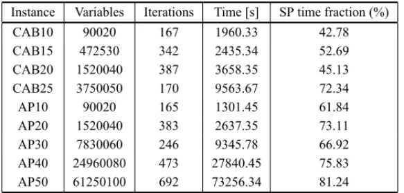
4.2 The GBD Algorithm Scalability
In order to test the performance of the deployed generalized Benders decomposition algorithm, the CAB data set of the US Civil Aeronautics Board and the AP data set introduced by Ernst and Krishnamoorthy [25, 27] have been used. The former includes problems with 10, 15, 20 and 25 nodes, while from the later problems with 10 to 200 nodes can be obtained.
The hub installation costs have been generated for all instances using a gaussian distribution with average equals to foand variance set to 40% to assess how the different fixed costs vary in real
problems. Where forepresents the scaled difference in objective value between a scenario in
which there is a virtual hub located in the center of mass and a scenario in which all nodes are hubs, as introduced by Eberyet al. [23]. For alternative works considering these test beds see [60, 24, 23, 7, 11, 10]. Furthermore, as done by Eberyet al. [23], the nodes with higher flows have been selected to have the higher fixed costs, hardening, in general, the selection of potential hubs.
The generalized Benders decomposition algorithm was implemented with the aid of the general purpose mixed integer programming package XPRESS-MP from Dash optimization. The pac-kage routines have been used on the solution of the mixed integer master program. The experi-ments have been carried out on a regular desktop micro-computer equipped with a Intel-Pentium IV 3.0 GHz processor and 2Gb of RAM memory. The value ofεhas been set to 0.0001%.
scenery of each iteration. In spite of this fact, some large problems could be solved in reasonable time, for a long term strategic decision problem.
Table 1– GBD algorithm scalability test.
Instance Variables Iterations Time [s] SP time fraction (%)
CAB10 90020 167 1960.33 42.78
CAB15 472530 342 2435.34 52.69
CAB20 1520040 387 3658.35 45.13
CAB25 3750050 170 9563.67 72.34
AP10 90020 165 1301.45 61.84
AP20 1520040 383 2637.35 73.11
AP30 7830060 246 9345.78 66.92
AP40 24960080 473 27840.45 75.83
AP50 61250100 692 73256.34 81.24
The large number of iterations is explained by the aggressive congestion cost functions that were adopted. For all these tests the parameterseandbwere taken as 0.5 and 2 respectively, implying a congestion cost ratio [10] scaling from 20% to 40%. Since GBD is an outer linearization strategy, it is particularly sensitive as the nonlinearities become dominant in a given MINLP.
4.3 Designing the Brazilian Air Transportation Network
Brazil is the fifth largest country of the world, and its area is 8.5 millions of squared kilometers, occupying about 47% of the area of South American continent. The population of the country is 184 million of inhabitants. Due to its great territorial extension and to the size its population, the country needs to have a great number of airports to allow the transportation of passengers and cargo. Nowadays, the country has 1759 private airports and 739 public airports, totaling 2498 airports.
Brazil is the second country of the world that more it possesses airports, behind just of the United States of America. The boards of INFRAERO and ANAC, two government agencies, are in charge of the management of 67 of those airports, that concentrate 97% of the commercial air transportation of the country. Those airports move about 2 million landings and takeoffs, and almost 50 million passengers and 1.2 million of tons per year (basis: year 2007).
In the last few years, Brazilian GDP is growing more than the average global GDP increase, around 5% year. This means an expected high demand increase for air transportation, since each 1% of increase on GDP means 1.15% of demand increase in the air transportation matrix. The passenger traffic in Brazil is strongly concentrated in few airports located in the cities of S ˜ao Paulo, Rio de Janeiro and Bras´ılia. The existent airports in those cities are the current passenger hubs of the Brazilian network.
and several flight cancelations. On the other hand, several other airports appear to have idle capacity, such as the airports in the cities of Belo Horizonte, Salvador and Curitiba.
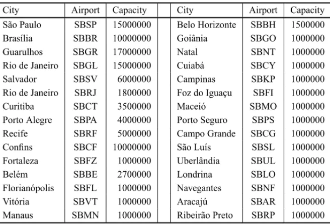
In order to use the deployed algorithms, several modeling assumptions have been made. Because of the large computational costs involved, only the 30 larger Brazilian airports were selected to compose the experience. Since INFRAERO and ANAC (Brazilian Civil Aeronautics Board) have historical series of the observed demands for each origin-destination pair in the network, as well as the distance matrix, the data mining phase was not a trouble. Another assumption was the use of the most economic available aircrafts, since the airlines always seek for the lowest operational costs.
The hub installation costs were estimated on the minimal infra-structure investment necessary to promote a node to the hub status. In some cases, this investment means only to improve air traffic control capabilities or to enlarge the passengers terminal or the cargo manipulation area. Sometimes this may imply to enlarge the runway length or to duplicate the existent runway or even to provide a better transportation system to reach the airport. These parameters were established according to the information provided by ANAC and INFRAERO.
Table 2– Hub nominal capacity array for the Brazilian case study (passengers/year).
City Airport Capacity City Airport Capacity
S˜ao Paulo SBSP 15000000 Belo Horizonte SBBH 1500000
Bras´ılia SBBR 10000000 Goiˆania SBGO 1000000
Guarulhos SBGR 17000000 Natal SBNT 1000000
Rio de Janeiro SBGL 15000000 Cuiab´a SBCY 1000000
Salvador SBSV 6000000 Campinas SBKP 1000000
Rio de Janeiro SBRJ 1800000 Foz do Iguac¸u SBFI 1000000
Curitiba SBCT 3500000 Macei´o SBMO 1000000
Porto Alegre SBPA 4000000 Porto Seguro SBPS 1000000
Recife SBRF 5000000 Campo Grande SBCG 1000000
Confins SBCF 10000000 S˜ao Lu´ıs SBSL 1000000
Fortaleza SBFZ 1000000 Uberlˆandia SBUL 1000000
Bel´em SBBE 2700000 Londrina SBLO 1000000
Florian´opolis SBFL 1000000 Navegantes SBNF 1000000
Vit´oria SBVT 1000000 Aracaj´u SBAR 1000000
Manaus SBMN 1000000 Ribeir˜ao Preto SBRP 1000000
In addition, a slightly different congestion function was used to account the congestion costs. For this set of experiences a function were the congestion effects are perceived only if a flow above 75% of the hub nominal capacity is reached was adopted:
τk(gk)=max0,e(gk−ak)b
A standard discount factorαof 0.5 for the inter-hub connections was adopted, since almost all the airlines establish a minimum of 50% of tickets sold by flight leg to be sustainable. The values of the parameterseandbwere taken as 1.0 and 2 producing very aggressive congestion effects (see [10]). To mimic the trend of growth of the traffic matrix, a triangular probability distribution was adopted, from 2011 to 2023. The central trend was taken forecasting a mean growth of 5.75% per year, corresponding to 5% of mean growth in GDP. The optimistic and pessimistic forecasts – the extremes of the triangular distribution – were based on the historical data from ANAC. Discrete distributions with ten sceneries were taken as approximations of the adopted triangular distributions. This small number of sceneries is necessary to ensure a reasonable computational cost, dealing with a little loss of accuracy.
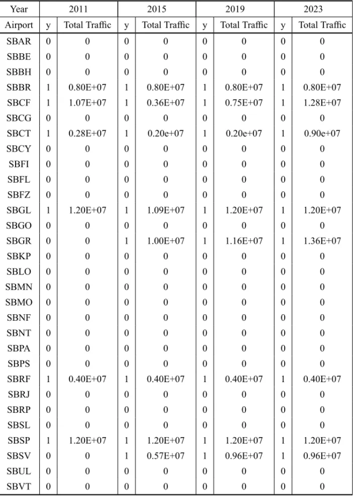
The obtained optimal hub structures – y vectors – and the expected total traffic for each hub are shown in Table 3. All the proposed instances have run in computing times under 15 hours of CPU. We must remark that only the flows on the hubs were displayed in Table 3, meaning that if a node is not a hub his traffic is not shown in Table 3. The resulting network designs are plotted graphically in Figures 1, 2, 3 and 4. In these figures, the relative thickness of a given link is a measure of its traffic intensity.
It is important to recall that the capacity array informs just the nominal capacities, since the true capacity of an airport is not known with accuracy. For instance, in 2007 SBSP has registered more than 18 millions of passengers, but its nominal capacity is only 15 millions. So, it is not unexpected to observe flows slightly above that nominal value, if it is preferable to tolerate some congestion to avoid the installation of new hubs. Other effect that is remarkable is the transfer of part of the increasing demand to the direct service links, as a way to save fixed or conges-tion costs. This flow transfer explains why the total hub traffic does not grows in the exact expected rate.
It is possible to see that the infrastructure investment may be directed to the airports of Belo Horizonte (SBCF), Recife (SBRF), Curitiba (SBCT) and Salvador (SBSV). These potential new hubs have idle capacity and may be better exploited in order to reduce the operational costs and flight delays on the Brazilian air transportation network. It is possible to see that it is also necessary to develop a strategy of expansion of all the network hubs, under penalty of a new traffic saturation in the near future. This expansion is particularly easy for SBCF and SBSV, complaining with data of INFRAERO and ANAC.
It was also observed an increasing transfer of traffic to the direct service links in order to avoid the hub congestion costs in 2019 and 2023, what recalls the urgency of a system expansion strategy. Another interesting effect is that the very huge traffic volume of the pair SBSP-SBRJ was not enough to make SBRJ a hub, since this particular airport has no capacity to deal with third party traffic.
Table 3– Computational Results for the Brazilian case.
Year 2011 2015 2019 2023
Airport y Total Traffic y Total Traffic y Total Traffic y Total Traffic
SBAR 0 0 0 0 0 0 0 0
SBBE 0 0 0 0 0 0 0 0
SBBH 0 0 0 0 0 0 0 0
SBBR 1 0.80E+07 1 0.80E+07 1 0.80E+07 1 0.80E+07
SBCF 1 1.07E+07 1 0.36E+07 1 0.75E+07 1 1.28E+07
SBCG 0 0 0 0 0 0 0 0
SBCT 1 0.28E+07 1 0.20e+07 1 0.20e+07 1 0.90e+07
SBCY 0 0 0 0 0 0 0 0
SBFI 0 0 0 0 0 0 0 0
SBFL 0 0 0 0 0 0 0 0
SBFZ 0 0 0 0 0 0 0 0
SBGL 1 1.20E+07 1 1.09E+07 1 1.20E+07 1 1.20E+07
SBGO 0 0 0 0 0 0 0 0
SBGR 0 0 1 1.00E+07 1 1.16E+07 1 1.36E+07
SBKP 0 0 0 0 0 0 0 0
SBLO 0 0 0 0 0 0 0 0
SBMN 0 0 0 0 0 0 0 0
SBMO 0 0 0 0 0 0 0 0
SBNF 0 0 0 0 0 0 0 0
SBNT 0 0 0 0 0 0 0 0
SBPA 0 0 0 0 0 0 0 0
SBPS 0 0 0 0 0 0 0 0
SBRF 1 0.40E+07 1 0.40E+07 1 0.40E+07 1 0.40E+07
SBRJ 0 0 0 0 0 0 0 0
SBRP 0 0 0 0 0 0 0 0
SBSL 0 0 0 0 0 0 0 0
SBSP 1 1.20E+07 1 1.20E+07 1 1.20E+07 1 1.20E+07
SBSV 0 0 1 0.57E+07 1 0.96E+07 1 0.96E+07
SBUL 0 0 0 0 0 0 0 0
SBVT 0 0 0 0 0 0 0 0
5 CONCLUDING REMARKS
In this article a model for accounting demand uncertainty and congestion costs for designing multiple allocation hub and spoke networks has been proposed. In addition, the proposed model allows the establishment of direct service links if they are economically interesting.
Generalized Benders decomposition was the selected technique to tackle the proposed problem. This technique has shown enough computing power to overcome large instances in reasonable time, although the computing times observed were expressively superior to those in [10], due to the most stressing congestion cost functions chosen.
The deployed algorithms were also used to redesign the Brazilian air transportation network, and the attained designs were properly discussed. The resulting network designs indicate that is necessary to redistribute flow on several hubs of the network in order to reduce the flight delays and other congestion effects. It has also pointed out that a system expansion is necessary in the near future under penalty of a new saturation of the installed infra-structure.
Future work must be devoted on evaluating how the capacity expansion of the major hubs may impact the proposed optimal hub-and-spoke networks.
ACKNOWLEDGEMENTS
We would like to thank the government of the state of Minas Gerais, Brazil, for partially suppor-ting this work. We also thank the traffic engineers Erivelton Guedes and Aur´elio Braga for the data and the insights they have provided from ANAC and INFRAERO. The authors’ research has been partially funded by CNPq, project 480757/2008-9, and FAPEMIG, project PPM-00399-09.
REFERENCES
[1] ALBAREDA-SAMBOLAM, FERNANDEZE & LAPORTEG. 2007. Heuristic and lower bound for a stochastic location-routing problem.European Journal of Operational Research,179(3): 940–955.
[2] ALUMUR S & KARA BY. 2008. Network hub location problems: The state of the art.European Journal of Operational Research,190: 1–21.
[3] AYKINT. 1994. Lagragian relaxation based approaches to capacitated hub-and-spoke network design problem.European Journal of Operational Research,79: 501–523.
[4] AYKINT. 1995. Network policies for hub-and-spoke systems with applications to the air transporta-tion system.Transportation Science,29: 201–221.
[5] BALAS E & BERGTHALLER C. 1983. Benders method revisited.Journal of Computational and Applied Mathematics,9: 3–12.
[6] BENDERSJF. 1962. Partitioning procedures for solving mixed-variables programming problems. Nu-merisch Mathematik,4: 238–252.
[8] CAIX, MCKINNEYDC, LASDONLS & WATKINSJRDW. 2001. Solving large nonconvex water resources management models using generalized Benders decompositon.Operations Research,49(2): 235–245.
[9] CAMARGORS, MIRANDAG & LUNA HPL. 2009. Benders decomposition for hub location pro-blems with economies of scale.Transportation Science,43: 86–97.
[10] CAMARGO RS DE, MIRANDA JR G, FERREIRA RPM & LUNA HP. 2009. Multiple allocation hub-and-spoke network design under hub congestion.Computers and Operations Research,36(12): 3097–3106.
[11] CAMARGORSDE, MIRANDAJRG & LUNAHP. 2008. Benders decomposition for the uncapaci-tated multiple allocation hub location problem.Computers and Operations Research,35(4): 1047– 1064.
[12] CAMPBELL JF. 1994. Integer programming formulations of discrete hub location problems.
European Journal of Operational Research,72: 387–405.
[13] CAMPBELLJF. 1994. A survey of network hub location.Studies in Locational Analysis,6: 31–49.
[14] CAMPBELLJF, ERNSTAT & KRISHNAMOORTHYM. 2002. Hub location problems. In: DREZNER Z & HAMACHERHW (Eds.).Facility Location: Application and Theory, pages 373–407. Springer.
[15] CAMPBELLJF, ERNST AT & KRISHNAMOORTHYM. 2005. Hub arc location problems: Part I – Introduction on results.Management Science,51(10): 1540–1555.
[16] CAMPBELLJF, ERNSTAT & KRISHNAMOORTHYM. 2005. Hub arc location problems: Part II – Formulations and optimal algorithms.Management Science,51(10): 1556–1571.
[17] CAMPBELLJF, STIEHRG, ERNST AT & KRISHNAMOORTHYM. 2003. Solving hub arc location problems on a cluster of workstations.Parallel Computing,29: 555–574.
[18] CAMPBELLJF. 1992. Location and allocation for distribution systems with transshipments and trans-portation economies of scale.Annals of Operations Research,40: 77–99.
[19] CANTOR DG & GERLA M. 1974. Optimal routing in a packet-swiched computer network.IEEE Transations on Computers,c-23(10): 1062–1069, October.
[20] CORDEAUJF, SOUMISF & DESROSIERSJ. 2000. A Benders decomposition approach for the loco-motive and car assignment problem.Transportation Science,34: 133–149.
[21] CORDEAUJF, SOUMISF & DESROSIERSJ. 2001. Simultaneous assignment of locomotives and cars to passenger trains.Operations Research,49(4): 531–548.
[22] COSTAMDAG, CAPTIVO ME & CL´IMACOJ. 2008. Capacitated single allocation hub location problem – a bi-criteria approach.Computers and Operations Research,35: 3671–3695.
[23] EBERYJ, KRISHNAMOORTHY M, ERNSTA & BOLANDN. 2000. The capacitated multiple allo-cation hub loallo-cation problema: Formulations and algorithms.European Journal of Operational Rese-arch,120: 614–631.
[24] ELHEDHLIS & HUFX. 2005. Hub-and-spoke network design with congestion.Computers & Ope-rations Research,32: 1615–1632.
[26] ERNST AT & KRISHNAMOORTHY M. 1998. Exact and heuristic algorithms for the uncapacitated multiple allocation p-hub median problem.European Journal of Operational Research,104: 100– 112.
[27] ERNSTAT & KRISHNAMOORTHYM. 1999. Solution algorithms for the capacitated single allocation hub location problem.Annals of Operations Research,86: 141–159.
[28] FRANC¸APM & LUNAHPL. 1982. Solving stochastic transportation-location problem by generali-zed benders decomposition.Transportation Science,16(2): 113–126.
[29] FRANKM & WOLFEP. 1956. An algorithm for quadratic programming.Naval Research Logistics Quarterly,3: 95–110.
[30] FRATTAM, GERLAM & KLEINROCKL. 1973. The flow deviation method: An approach to store-and-forward communication network design.Networks,3: 97–133.
[31] GABOR AF & VAN OMMEREN JCW. 2006. An approximation algorithm for a facility location problem with stochastic demands and inventories.Operations Research Letters,34(3): 257–263.
[32] GEOFFRIONAM & GRAVESGW. 1974. Multicomodity distribution system design by Benders de-composition.Management Science,20: 822–844.
[33] GEOFFRIONAM. 1972. Generalized Benders decomposition.Journal of optimization Theory and Applications,10(4): 237–260.
[34] GERLAM. 1973.The Design of Store-and-Forward (S/F) Networks for Computer Communications. PhD thesis, University of California, Los Angeles, EUA.
[35] GILLEND & LEVINSOND. 1999. The full cost of air travel in the california corridor. In: PRESEN
-TED IN THE78thANNUALMEETING OFTRANSPORTATIONRESEARCHBOARD, Washington, DC, January, 10–14.
[36] GROVE GP & O’KELLY ME. 1986. Hub networks and simultated schedule delay.Papers of the Regional Science Association,59: 103–119.
[37] HAMACHERHW, LABBE´ M, NICKELS & SONNEBORNT. 2004. Adapting polyhedral properties from facility to hub location problems.Discrete Applied Mathematics,145: 104–116.
[38] HERAGUSS & CHENJ-S. 1998. Optimal solution of cellular manufacturing system design: Benders decomposition approach.European Journal of Operational Research,107: 175–192.
[39] HOANGHH. 2005. Topological optimization of networks: A nonlinear mixed integer model em-ploying generalized benders decomposition.IEEE Transations on Automatic Control,AC-27: 164– 169.
[40] HOCHREITERR & PFLUGGC. 2007. Financial scenario generation for stochastic multistage deci-sion processes as facility location problems.Annals of Operations Research,152: 257–272.
[41] KARABY & TANSELBC. 2003. The latest arrival hub location problem.Management Science,47: 1408–1420.
[42] KLINCEWICZ JG. 1998. Hub location in backbone/tributary network design: a review. Location Science,6: 307–335.