ISSN 0101-8205 www.scielo.br/cam
New versions of the Hestenes-Stiefel nonlinear
conjugate gradient method based on the secant
condition for optimization
LI ZHANG
College of Mathematics and Computational Science Changsha University of Science and Technology
Changsha 410076, China E-mail: [email protected]
Abstract. Based on the secant condition often satisfied by quasi-Newton methods, two new versions of the Hestenes-Stiefel (HS) nonlinear conjugate gradient method are proposed, which are descent methods even with inexact line searches. The search directions of the proposed methods have the formdk = −θkgk+βkH Sdk−1, ordk = −gk+βkH Sdk−1+θkyk−1. When
exact line searches are used, the proposed methods reduce to the standard HS method. Conver-gence properties of the proposed methods are discussed. These results are also extended to some other conjugate gradient methods such as the Polak-Ribiére-Polyak (PRP) method. Numerical results are reported.
Mathematical subject classification: 90C30, 65K05.
Key words:HS method, descent direction, global convergence.
1 Introduction
Assume that f: Rn→ Ris a continuously differentiable function whose gradi-ent is denoted byg. The problem considered in this paper is
min f(x), x ∈ Rn. (1.1)
The iterates for solving (1.1) are given by
xk+1=xk +αkdk, (1.2)
where the stepsizeαk is positive and computed by some line search, and dk is
the search direction.
Conjugate gradient methods are very efficient iterative methods for solving (1.1) especially whennis large. The search direction has the following form:
dk = (
−gk, if k =0, −gk+βkdk−1, if k >0,
(1.3)
where βk is a parameter. Some well-known conjugate gradient methods
in-clude the Polak-Ribiére-Polyak (PRP) method [17, 18], the Hestenes-Stiefel (HS) method [13], the Liu-Storey (LS) method [15], the Fletcher-Reeves (FR) method [8], the Dai-Yuan (DY) method [5] and the conjugate descent (CD) method [9]. In this paper, we are interested in the HS method, in which βk is
defined by
βkH S= g T k yk−1 dT
k−1yk−1
, (1.4)
whereyk−1=gk−gk−1. Throughout the paper, we denotesk−1=xk−xk−1=
αk−1dk−1, andk ∙ k stands for the Euclidean norm. Convergence properties of conjugate gradient methods can be found in the book [6], the survey paper [12] and references therein.
The HS method behaves like the PRP method in practical computation and is generally regarded as one of the most efficient conjugate gradient methods. An important feature of the HS method is that it satisfies conjugacy condition
dkTyk−1=0, (1.5)
which is independent of the objective function and line search. However, Dai and Liao [4] pointed out that in the casegkT+1dk 6= 0, the conjugacy condition
(1.5) may have some disadvantages (for instance, see [21]). In order to construct a better formula forβk, Dai and Liao proposed a new conjugacy condition and a
new conjugate gradient method called the Dai-Liao (DL) method, given by
βkD L = g T
k yk−1−tsk−1
dkT−1yk−1
(1.6)
Besides conjugate gradient methods, the following gradient type methods
dk = (
−gk, if k =0, −θkgk+βkdk−1, if k >0,
(1.7)
have also been studied extensively by many authors. Hereθk andβk are two
parameters. Clearly, ifθk = 1, the methods (1.7) become conjugate gradient
methods (1.3). When
βk =
θkyk−1−sk−1
T
gk
dkT−1yk−1
,
the methods (1.7) reduce to spectral conjugate gradient methods [2] and scaled conjugate gradient methods [1]. Yuan and Stoer [21] proposed a subspace method to compute the parameters θk and βk which solve the following
sub-problem
min
d∈k
φk(d)=gkTd+
1 2d
TB kd,
wherek = Span{gk,dk−1}and Bk is a suitable quasi-Newton matrix such as
the memoryless BFGS update matrix [19]. Zhang et al. [23] proposed a modi-fied FR method where the parameters in (1.7) are given by
θk =
dkT−1yk−1
kgk−1k2
, βk =βkF R = kgkk2 kgk−1k2
.
This method satisfiesgT
kdk = −kgkk2and this property depends neither on the
line search used, nor on the convexity of the objective function. Moreover, this method converges globally for nonconvex functions with Armijo or Wolfe line search.
Recently, based on the direction generated by the memoryless BFGS update matrix [19], Zhang et al. [22, 24] proposed the following three-term conjugate gradient type method,
dk = (
−gk, if k =0,
−gk+βkdk−1+θkyk−1, if k >0,
(1.8)
whereθkandβk are two parameters. If the parameters in (1.8) are given by
βk =βkP R P =
gkTyk−1
kgk−1k2
, θk = −
gkTdk−1
kgk−1k2
then this method becomes the modified PRP method [22]. If the parameters in (1.8) are chosen as
βk =βkH S, θk = − gkTdk−1
dT k yk−1
,
then we get the three-term HS method [24]. Both methods still retain the rela-tiongT
kdk = −kgkk2and performed well in practical computations.
In this paper, we are concerned with the methods (1.7) and (1.8) with the parameterβk =βkH S. Then we try to construct newθk by using idea of the DL
method [4].
This paper is organized as follows. In Section 2, we present new formulas forθk and corresponding algorithms. In Section 3, we analyze global
conver-gence properties of the proposed methods with some inexact line searches. In Section 4, we extend the results of Section 2 and Section 3 to other conjugate gradient methods. In Section 5, we report numerical comparisons with existing conjugate gradient methods by using problems in the CUTE library [3].
2 New formula forθk and algorithms
In this section, we first describe the following two-terms HS conjugate gradient type method,
dk = (
−gk, if k =0,
−(1+θk′)gk+βkH Sdk−1, if k >0,
(2.1)
where, for convenience, we writeθk =1+θk′.
In order to introduce our method, let us simply recall the conjugacy condition proposed by Dai and Liao [4]. Linear conjugate gradient methods generate a search direction such that the conjugacy condition holds, namely,
diTQdj =0 ∀i6= j,
whereQis the symmetric and positive definite Hessian matrix of the quadratic objective function f(x). For general nonlinear functions, it follows from the mean value theorem that there exists someτ ∈(0,1)such that
dkTyk−1=αk−1dkT∇
2
f xk−1+τ αk−1dk−1
Therefore it is reasonable to replace (2.2) by the following conjugacy condition:
dkTyk−1=0. (2.3)
Dai and Liao [4] used the secant condition of quasi-Newton methods, that is,
Hkyk−1=sk−1, (2.4)
where Hk is an approximation to the inverse Hessian. For quasi-Newton
methods, the search directiondkcan be calculated in the form
dk = −Hkgk. (2.5)
By the use of (2.4) and (2.5), we get that
dkTyk−1= − Hkgk T
yk−1= −gTk Hkyk−1
= −gkTsk−1.
The above relation implies that (2.3) holds if the line search is exact since in this casegTksk−1 =0. However, practical numerical algorithms normally adopt inexact line searches instead of exact ones. For this reason, Dai and Liao replaced the above conjugacy condition by
dkTyk−1= −tgkTsk−1, (2.6)
wheretis a scalar. If we substitute (1.3) into (2.6), we get the formula forβkD L
in (1.6).
In order to get the formula forθk in our method, substituting (2.1) into (2.6),
we have
θk′gkTyk−1=tgkTsk−1. Set
t =hgkTyk−1,
wherehis a parameter. We get from the above two equalities that
θk′ =hgTksk−1.
Now let
h= g
T kyk−1
skT−1yk−1kgkk2
− ρ
skT−1yk−1
withρ∈ [0,1]. Then, we have
θk′ =βkH Sg
T kdk−1
kgkk2
−ρ g
T kdk−1
dkT−1yk−1
.
For convenience, we summarize the above method as the following algorithm which we call the two-term HS method.
Algorithm 2.1(two-term HS Method):
Step 0: Given the constantρ ∈ [0,1], choose an initial point x0 ∈ Rn. Letk :=0.
Step 1:Computedk by
dk = (
−gk, if k=0, −θkgk+βkH Sdk−1, if k>0,
(2.7)
where
θk =1+θk′ =1+β H S k
gT kdk−1
kgkk2 −ρ
gT kdk−1
dkT−1yk−1
. (2.8)
Step 2:Determineαkby some line search.
Step 3:Let the next iterate bexk+1=xk+αkdk.
Step 4:Letk :=k+1. Go to Step 1.
By the same argument as Algorithm 2.1, we can get the following three-term HS method. In the rest of this paper, we only give the direction in the algorithm where the other steps are as same as Algorithm 2.1 since conjugate gradient methods are mainly determined by their search directions.
Algorithm 2.2(three-term HS Method):
dk = (
−gk, if k =0,
−gk+βkH Sdk−1+θ (1)
k yk−1, if k >0,
(2.9)
where
θk(1) =ρ kgkk
2
gkTyk−1
gkTdk−1
dkT−1yk−1
− g T kdk−1
dkT−1yk−1
Remark 2.1. It is interesting to note that when ρ = 0 in (2.7)–(2.8) or (2.9)–(2.10), we have
dkTgk = −kgkk2−βkH Sg T
kdk−1+βkH Sg T
kdk−1= −kgkk2,
which is independent of any line search and convexity of the objective function. In this case, Algorithm 2.2 reduces to the three-term HS method [24].
Remark 2.2. If exact line search is used, it is easy to see that Algorithm 2.1 and Algorithm 2.2 reduce to the standard HS method.
3 Convergence properties
In this section, we only analyze convergence properties of Algorithm 2.1. The corresponding results for Algorithm 2.2 can be obtained by using same argument as Algorithm 2.1. In the global convergence analysis of many iterative methods, the following assumption is often needed.
Assumption A.
(i) The level set= {x ∈ Rn|f(x)≤ f(x0)}is bounded.
(ii) In some neighborhood N of , f is continuously differentiable and its gradient is Lipschitz continuous, namely, there exists a constant L > 0 such that
kg(x)−g(y)k ≤Lkx−yk, ∀x,y ∈ N. (3.1)
Clearly, Assumption A implies that there exists a constantγ such that
kg(x)k ≤γ , for all x ∈ N. (3.2)
In order to ensure global convergence of Algorithm 2.1, we need some line search to compute the stepsize αk. The Wolfe line search consists of finding
αk satisfying
(
f(xk+αkdk)≤ f(xk)+δαkgkTdk,
dkTg(xk +αkdk)≥σdkTgk.
The strong Wolfe line search corresponds to: that
(
f(xk+αkdk)≤ f(xk)+δαkgkTdk,
|dT
k g(xk+αkdk)| ≤ |σdkTgk|,
(3.4)
where 0< δ < σ <1 are constants.
The following lemma, called the Zoutendijk condition, is often used to prove global convergence of conjugate gradient methods. It was originally given by Zoutendijk [25] and Wolfe [20].
Lemma 3.1. Let Assumption A hold,{xk}be generated by(1.2)and dk satisfy gT
kdk <0. Ifαksatisfies the Wolfe condition(3.3)or the strong Wolfe condition
(3.4), then we have
∞
X
k=0
(gT kdk)
2
kdkk2 <+∞. (3.5)
In the global convergence analysis for many methods, the sufficient descent condition plays an important role. The following result shows that Algorithm 2.1 produces sufficient descent directions.
Lemma 3.2. Let{xk}and{dk}be generated by Algorithm 2.1, and letαk be obtained by the Wolfe line search(3.4). Ifρ ∈ [0,1), then we have
gT kdk kgkk2
≤ −(1−ρ). (3.6)
Moreover, ifρ=1, then gkTdk <0.
Proof. We have from (2.7) and the definition ofβkH S (1.4) that
gkTdk = −kgkk2+ρ
gkTdk−1
dT k−1yk−1
kgkk2, (3.7)
which implies that
gT kdk
kgkk2 = −1+ρ
gT kdk−1 dT
k−1yk−1
= −(1−ρ)−ρ+ρ g
T kdk−1 dT
k−1yk−1
= −(1−ρ)+ρg
T k−1dk−1
dkT−1yk−1
.
Since
g0Td0= −kg0k2<0 and the Wolfe line search implies
d0Ty0≥(1−σ )kg0k2>0,
from (3.8), we have (3.6) by induction. The proof is then finished.
By the use of the first equality in (3.8) and the second inequality in the strong Wolfe line search (3.4), we have the following result.
Lemma 3.3. Let{xk}and{dk}be generated by Algorithm 2.1, and letαk be obtained by the strong Wolfe line search(3.4)withσ < 12. Ifρ = 1, then we have
gkTdk kgkk2
≤ −1−2σ
1−σ . (3.9)
The following theorem establishes global convergence of Algorithm 2.1 for strongly convex functions.
Theorem 3.4. Suppose Assumption A holds and f is strongly convex on N , that is, there exists a constantμ >0such that
(g(x)−g(y))T(x−y)≥μkx−yk2, ∀x,y∈ N. (3.10)
Ifρ ∈ [0,1), then the sequence{xk}generated by Algorithm2.1with the Wolfe line search(3.3)satisfieslimk→∞kgkk =0.
Proof. It follows from (3.10) and (3.1) that
LdkT−1sk−1≥dkT−1yk−1≥μdkT−1sk−1. (3.11)
Now we begin to estimateθk andβk in (2.7). It follows from (1.4), (3.1) and
(3.11) that
|βkH S| =
gTkyk−1
dT k−1yk−1
≤
Lkgkkksk−1k
μdT k−1sk−1
= Lkgkk
μkdk−1k
It follows from (2.8), (3.12) and the second inequality in (3.3) that
|θk| =
1−ρ+β H S k
gkTdk−1
kgkk2 −ρg
T k−1dk−1
dT k−1yk−1
≤ 1−ρ+ |βkH S|kgkkkdk−1k kgkk2
+ ρ|g T k−1dk−1|
(1−σ )|gT k−1dk−1|
≤ 1−ρ+ L
μ + ρ
1−σ.
The above inequality together with (3.12) implies that
kdkk ≤ |θk|kgkk + |βkH S|kdk−1k
≤
1−ρ+2L
μ + ρ
1−σ
kgkk=△ Mkgkk.
(3.13)
We have from (3.6) and (3.5) that
∞
X
k=0
kgkk4 kdkk2
<∞.
It follows from the above inequality and (3.13) that
∞
X
k=0
kgkk2<∞,
which means limk→∞kgkk =0. The proof is then completed.
By Lemma 3.3 and same argument in the above theorem, we have the follow-ing corollary.
Corollary 3.5. Suppose Assumption A holds and f is strongly convex on N . If
ρ = 1andαk is determined by the strong Wolfe line search(3.4)withσ < 12, then the sequence{xk}generated by Algorithm2.1satisfieslimk→∞kgkk =0.
In order to ensure global convergence of Algorithm 2.1 for nonconvex func-tions, we adopt the idea of the MBFGS method proposed by Li and Fukushi-ma [14] and modify Algorithm 2.1, replacingyk−1in (2.7) by
Algorithm 3.1(modified two-term HS Method):
dk = (
−gk, if k =0,
−θkM H Sgk+βkM H Sdk−1, if k >0,
(3.15)
where
βkM H S = g T kzk−1
dT k−1zk−1
, θkM H S =1+βkM H Sg
T kdk−1
kgkk2
−ρ g
T kdk−1
dT k−1zk−1
. (3.16)
An important property of zk−1 is that, when the Wolfe line search is used, it satisfies
L+ε1
dkT−1sk−1≥dkT−1zk−1≥ε1dkT−1sk−1. (3.17) This inequality is the same as (3.11) and plays the same role in the proof of global convergence of Algorithm 3.1 for nonconvex functions. By the use of (3.17) and the same arguments as in Theorem 3.4, we have the following strongly global convergence result for Algorithm 3.1 for nonconvex objective functions.
Theorem 3.6. Suppose Assumption A holds, then the sequence{xk}generated by Algorithm3.1with the Wolfe line search(3.3)satisfieslimk→∞kgkk =0.
Another technique to guarantee global convergence of conjugate gradient methods for general nonlinear functions is to restrictβk nonnegative as in the
PRP+ and HS+ methods [10]. In fact, if we replaceβkH S in Algorithm 2.1 by
βkH S+=max{0, βkH S},we have the following algorithm which we call the two-term HS+ Method.
Algorithm 3.2(two-term HS+ Method):
dk = (
−gk, if k =0,
−θkH S+gk+βkH S+dk−1, if k >0,
(3.18)
where
θkH S+=1+βkH S+g
T kdk−1
kgkk2
−ρ g
T kdk−1
dkT−1yk−1
. (3.19)
Theorem 3.7. Suppose Assumption A holds, then the sequence{xk}generated by Algorithm3.2with the strong Wolfe line search(3.4)satisfies
lim inf
k→∞ kgkk =0.
4 Applications
In this section, we extend the results on new versions of the HS method in Sections 2 and 3 to some well-known conjugate gradient methods. For instance, if we replace the termdT
k−1yk−1in step 1 of Algorithm 2.1 and Algorithm 2.2 by kgk−1k2 or−dkT−1gk−1, we get new versions of the PRP and LS methods, respectively.
Algorithm 4.1(two-term PRP Method):
dk = (
−gk, if k=0,
−θkP R P1gk +βkP R Pdk−1, if k>0,
(4.1)
where
θkP R P1=1+βkP R Pg
T kdk−1 kgkk2
−ρg
T kdk−1 kgk−1k2
. (4.2)
Algorithm 4.2(three-term PRP Method):
dk = (
−gk, if k =0,
−gk +βkP R Pdk−1+θkP R P2yk−1, if k >0, where
θkP R P2=ρ kgkk
2
gT k yk−1
gT kdk−1 kgk−1k2
− g T kdk−1 kgk−1k2
.
Algorithm 4.3(two-term LS Method):
dk = (
−gk, if k =0, −θkL S1gk +βkL Sdk−1, if k >0, where
βkL S = − g T k yk−1
dkT−1gk−1
, θkL S1=1+βkL Sg
T kdk−1
kgkk2
+ρ g
T kdk−1
dkT−1gk−1
Algorithm 4.4(three-term LS Method):
dk = (
−gk, if k=0,
−gk+βkL Sdk−1+θkL S2yk−1, if k>0, where
θkL S2= −ρ kgkk
2
gT k yk−1
gkTdk−1
dT k−1gk−1
+ g T kdk−1
dT k−1gk−1
.
Algorithm 4.5(two-term FR Method):
dk = (
−gk, if k=0, −θkF Rgk+βkF Rdk−1, if k>0,
(4.3)
where
θkF R=1+βkF Rg
T kdk−1
kgkk2 −ρg
T kdk−1
kgk−1k2
. (4.4)
Remark 4.1. Whenρ=0 in the above algorithms, the search direction satisfies the sufficient descent conditiondT
k gk = −kgkk2,which is also independent of
any line search and convexity of the objective function. Moreover in this case, Algorithms 4.2 and 4.3 are identical and reduce to the modified PRP method [23], and Algorithm 4.5 becomes the modified FR method [22]. It is clear that these methods reduce to conjugate gradient methods respectively if exact line search is used.
Remark 4.2. Global convergence properties of these algorithms are similar to those of Algorithm 2.1 or Algorithm 2.2. Here we only analyze Algorithm 4.1 and Algorithm 4.5.
The next result shows that the direction generated by Algorithm 4.1 or Algo-rithm 4.5 satisfies the sufficient descent condition if the strong Wolfe line search (3.4) is used.
Lemma 4.1. Let{xk}and{dk}be generated by Algorithm4.1or Algorithm4.5 with the strong Wolfe line search(3.4). Ifρ < 2σ1, then for all k, we have that
−1−(ρσ ) k
1−ρσ ≤
gkTdk kgkk2
≤ −1−2ρσ +(ρσ ) k
1−ρσ ≤ −
1−2ρσ
problem ρ iter fn gn kg(x)k∞ f(x) time
DIXMAANI 0.0 3459 6919 3460 0.9641D-06 0.1000D+01 13.58 ( 6000) 0.2 3376 6753 3377 0.9525D-06 0.1000D+01 12.95 0.4 3241 6483 3242 0.9934D-06 0.1000D+01 12.44 0.6 3074 6149 3075 0.9505D-06 0.1000D+01 11.79 0.8 2927 5855 2928 0.9941D-06 0.1000D+01 11.22 1.0 2870 5741 2871 0.9970D-06 0.1000D+01 11.01 TRIDIA 0.0 1115 2231 1116 0.9932D-06 0.4211D-14 2.92 (10000) 0.2 1115 2231 1116 0.9907D-06 0.4216D-14 3.71 0.4 1115 2231 1116 0.9982D-06 0.4181D-14 2.91 0.6 1116 2233 1117 0.9628D-06 0.3884D-14 2.93 0.8 1115 2231 1116 0.9982D-06 0.4185D-14 2.93 1.0 1115 2231 1116 0.9681D-06 0.4176D-14 2.92 CURLY30 0.0 10769 17008 17441 0.8923D-06 -0.1003D+06 10.01 ( 1000) 0.2 9993 16126 15621 0.8650D-06 -0.1003D+06 8.76
0.4 10706 16996 17134 0.8343D-06 -0.1003D+06 9.51 0.6 10065 16310 15707 0.9882D-06 -0.1003D+06 8.84 0.8 9854 15998 15246 0.9443D-06 -0.1003D+06 8.61 1.0 9808 15994 15012 0.9442D-06 -0.1003D+06 8.52 CURLY10 0.0 10853 16209 17260 0.9280D-06 -0.1003D+06 5.05 ( 1000) 0.2 10867 16213 17244 0.9981D-06 -0.1003D+06 4.86 0.4 10660 15986 16848 0.8842D-06 -0.1003D+06 4.80 0.6 10781 16127 17078 0.9710D-06 -0.1003D+06 4.85 0.8 10743 16062 16999 0.9429D-06 -0.1003D+06 4.84 1.0 10732 15957 17087 0.9225D-06 -0.1003D+06 4.84 EIGENALS 0.0 2755 5516 2767 0.8979D-06 0.4309D-10 26.27 ( 930) 0.2 2921 5848 2934 0.5473D-06 0.3583D-10 21.69 0.4 2603 5212 2615 0.7806D-06 0.6556D-10 19.68 0.6 2838 5682 2848 0.8246D-06 0.5192D-10 21.07 0.8 2639 5284 2653 0.9181D-06 0.2030D-10 19.98 1.0 2704 5414 2715 0.5283D-06 0.3591D-10 20.04 FMINSURF 0.0 607 1218 611 0.9973D-06 0.1000D+01 5.54 (10000) 0.2 629 1259 630 0.8559D-06 0.1000D+01 5.29 0.4 609 1219 610 0.8983D-06 0.1000D+01 5.12 0.6 601 1203 602 0.9117D-06 0.1000D+01 5.07 0.8 600 1201 601 0.8677D-06 0.1000D+01 5.07 1.0 590 1182 592 0.9383D-06 0.1000D+01 4.97 BDQRTIC 0.0 10006 14943 21460 0.8604D-06 0.4003D+05 116.72 (10000) 0.2 2031 4188 3071 0.9234D-06 0.4003D+05 20.47
0.4 2636 5530 4672 0.9835D-06 0.4003D+05 29.34 0.6 1359 2986 2498 0.8684D-06 0.4003D+05 15.85 0.8 1247 2733 2394 0.8808D-06 0.4003D+05 14.18 1.0 1879 4036 4982 0.9410D-06 0.4003D+05 27.80 FMINSRF2 0.0 423 848 425 0.9950D-06 0.1000D+01 3.73 (10000) 0.2 435 871 436 0.9353D-06 0.1000D+01 3.86 0.4 420 841 421 0.9953D-06 0.1000D+01 3.45 0.6 420 841 421 0.9892D-06 0.1000D+01 3.46 0.8 426 853 427 0.8962D-06 0.1000D+01 3.51 1.0 420 841 421 0.8994D-06 0.1000D+01 3.46
problem ρ iter fn gn kg(x)k∞ f(x) time
FMINSRF2 0.0 495 995 500 0.9745D-06 0.1000D+01 7.53 (15625) 0.2 497 997 500 0.9647D-06 0.1000D+01 6.76 0.4 507 1015 508 0.9508D-06 0.1000D+01 7.07 0.6 491 984 493 0.9896D-06 0.1000D+01 6.70 0.8 515 1031 516 0.9639D-06 0.1000D+01 6.86 1.0 492 985 493 0.8987D-06 0.1000D+01 6.54 TESTQUAD 0.0 2213 4427 2214 0.8599D-06 0.2117D-12 5.50 (10000) 0.2 2227 4455 2228 0.9356D-06 0.2108D-12 5.07 0.4 2169 4339 2170 0.9682D-06 0.7841D-12 4.83 0.6 2232 4465 2233 0.8829D-06 0.2106D-12 4.91 0.8 2175 4351 2176 0.9072D-06 0.7838D-12 4.77 1.0 2234 4469 2235 0.8896D-06 0.2107D-12 4.90
Table 1 – (continuation).
Proof. We prove (4.5) by induction. SincegT
0d0 = −kg0k
2, in this case, the relation (4.5) holds withk =0. It follows from (4.1) or (4.3) that
gTkdk kgkk2
= −1+ρg
T kdk−1 kgk−1k2
. (4.6)
The above equality with the second inequality in (3.4) implies that
−1+ρσg
T k−1dk−1
kgk−1k2
≤ g T kdk
kgkk2 ≤ −1−ρσ
gT k−1dk−1
kgk−1k2
.
Repeating the same process, we have that
−
1+ρσ+(ρσ )2+∙ ∙ ∙+(ρσ )k−1
≤ g
T kdk kgkk2
≤ −1+ρσ+(ρσ )2+∙ ∙ ∙+(ρσ )k−1,
which shows that (4.5) holds. The proof is then completed.
Remark 4.3. If we replaceβP R P
k in Algorithm 4.1 byβ P R P+
k =max{0, βkP R P},
then this restricted algorithm converges globally for nonconvex functions by Lemma 4.1 and the argument of Theorem 4.3 in [10].
The next result is based on the work of [23]. Here we also omit its proof.
cg-descent Algorithm 2.1 prp+
problem n iter / fn / gn /time iter / fn / gn /time iter / fn / gn /time
FLETCHCR 5000 31998/66391/34677/ 102.18 20046/40142/20108/ 59.04 19987/40000/40000/ 83.00
CURLY30 1000 9765/15713/15122/ 8.51 9808/15994/15012/ 8.45 -1/-1/-1/-1.00
CURLY20 1000 9757/15481/15084/ 6.75 10644/16517/17037/ 7.22 -1/-1/-1/-1.00
DIXMAANI 6000 2660/ 5321/ 2661/ 10.65 2870/ 5741/ 2871/ 11.10 2357/ 4720/ 4720/ 14.10
EIGENBLS 420 4970/ 9947/ 4978/ 9.39 4615/ 9236/ 4623/ 8.54 4832/ 9714/ 9714/ 14.91
TRIDIA 10000 1115/ 2231/ 1116/ 3.02 1115/ 2231/ 1116/ 3.22 1114/ 2231/ 2231/ 3.91
NONDQUAR 5000 5012/10050/ 5099/ 7.43 2994/ 6004/ 3104/ 4.25 5006/10058/10058/ 9.52
CURLY10 1000 9431/14475/14406/ 4.48 10732/15957/17087/ 4.81 -1/-1/-1/-1.00
EIGENCLS 462 1776/ 3575/ 1802/ 3.94 1729/ 3467/ 1741/ 3.98 1650/ 3312/ 3312/ 6.00
SPARSINE 1000 4515/ 9031/ 4516/ 4.17 6091/12183/ 6092/ 6.06 4394/ 8793/ 8793/ 6.44
EIGENALS 420 1329/ 2665/ 1344/ 2.52 1336/ 2679/ 1353/ 2.73 1482/ 2998/ 2998/ 4.63
FLETCHCR 1000 6828/14236/ 7479/ 3.99 4939/ 9987/ 5062/ 2.41 4471/ 8986/ 8986/ 3.37
GENHUMPS 1000 3344/ 6857/ 3555/ 6.35 2486/ 5046/ 2580/ 4.33 2719/ 5807/ 5807/ 7.48
FMINSURF 5625 491/ 983/ 492/ 2.14 475/ 954/ 479/ 2.31 471/ 949/ 949/ 3.25
TRIDIA 5000 782/ 1565/ 783/ 0.79 782/ 1565/ 783/ 0.86 781/ 1565/ 1565/ 1.29
DIXMAANE 6000 302/ 605/ 303/ 1.23 306/ 613/ 307/ 1.32 307/ 620/ 620/ 2.09
DIXMAANJ 6000 295/ 591/ 296/ 1.25 311/ 623/ 312/ 1.32 275/ 557/ 557/ 1.99
BDQRTIC 5000 3763/ 6992/ 8726/ 22.78 1706/ 3547/ 2102/ 6.90 -1/-1/-1/-1.00
DIXMAANK 6000 263/ 527/ 264/ 1.05 314/ 629/ 315/ 1.23 289/ 587/ 587/ 1.77
NONCVXU2 1000 1928/ 3731/ 2055/ 2.14 1942/ 3785/ 2043/ 1.80 1956/ 3919/ 3919/ 2.81
DIXMAANL 6000 244/ 489/ 245/ 1.02 264/ 529/ 265/ 1.09 346/ 702/ 702/ 2.65
SENSORS 100 25/ 57/ 44/ 0.78 31/ 67/ 49/ 0.95 27/ 66/ 66/ 1.17
DIXMAANF 6000 229/ 459/ 230/ 0.98 223/ 447/ 224/ 1.02 215/ 437/ 437/ 1.62
DIXMAANG 6000 226/ 453/ 227/ 0.96 228/ 457/ 229/ 0.96 206/ 420/ 420/ 1.81
DIXMAANH 6000 223/ 447/ 224/ 0.95 218/ 437/ 219/ 0.93 408/ 825/ 825/ 2.97
FLETCBV2 1000 1052/ 2105/ 1055/ 0.94 1222/ 2445/ 1225/ 1.06 942/ 1886/ 1886/ 1.50
SCHMVETT 10000 41/ 68/ 60/ 1.37 50/ 87/ 73/ 1.64 44/ 105/ 105/ 2.45
GENHUMPS 500 1940/ 4132/ 2258/ 1.90 2032/ 4179/ 2171/ 1.82 1896/ 4147/ 4147/ 2.60
CRAGGLVY 5000 111/ 204/ 143/ 0.98 110/ 204/ 150/ 1.19 -1/-1/-1/-1.00
MOREBV 10000 95/ 191/ 97/ 0.67 106/ 213/ 108/ 0.77 100/ 201/ 201/ 1.33
WOODS 10000 187/ 426/ 257/ 1.18 224/ 491/ 283/ 1.31 232/ 487/ 487/ 2.15
NONDQUAR 1000 2958/ 5924/ 3147/ 0.87 3059/ 6128/ 3291/ 0.87 4015/ 8128/ 8128/ 1.51
SPARSQUR 10000 22/ 45/ 23/ 0.37 34/ 69/ 35/ 0.53 41/ 131/ 131/ 1.42
POWER 5000 258/ 517/ 259/ 0.31 262/ 525/ 263/ 0.29 252/ 514/ 514/ 0.40
MANCINO 100 11/ 23/ 12/ 0.66 12/ 25/ 13/ 0.71 11/ 27/ 27/ 1.09
CRAGGLVY 2000 106/ 191/ 132/ 0.35 108/ 200/ 140/ 0.37 -1/-1/-1/-1.00
CURLY30 200 1920/ 3515/ 2819/ 0.33 1810/ 3330/ 2594/ 0.30 -1/-1/-1/-1.00
LIARWHD 10000 25/ 60/ 41/ 0.42 19/ 40/ 24/ 0.34 15/ 46/ 46/ 0.41
BDQRTIC 1000 628/ 1296/ 1025/ 0.56 416/ 878/ 572/ 0.35 -1/-1/-1/-1.00
GENROSE 500 1259/ 2559/ 1309/ 0.33 1163/ 2350/ 1207/ 0.26 1123/ 2278/ 2278/ 0.36
VARDIM 10000 50/ 109/ 62/ 0.31 52/ 138/ 91/ 0.34 -1/-1/-1/-1.00
CURLY20 200 1998/ 3546/ 2951/ 0.28 1895/ 3386/ 2769/ 0.25 -1/-1/-1/-1.00
FREUROTH 5000 65/ 126/ 96/ 0.48 69/ 134/ 108/ 0.52 -1/-1/-1/-1.00
ENGVAL1 10000 25/ 43/ 35/ 0.36 25/ 47/ 35/ 0.37 -1/-1/-1/-1.00
POWELLSG 10000 64/ 130/ 77/ 0.29 187/ 378/ 216/ 0.62 165/ 362/ 362/ 0.73
DIXON3DQ 1000 1000/ 2001/ 1002/ 0.26 1000/ 2001/ 1002/ 0.24 1000/ 2005/ 2005/ 0.33
BRYBND 5000 36/ 74/ 39/ 0.31 32/ 66/ 35/ 0.28 26/ 66/ 66/ 0.38
HILBERTA 200 40/ 81/ 50/ 0.45 16/ 33/ 21/ 0.29 15/ 38/ 38/ 0.35
TQUARTIC 10000 25/ 77/ 61/ 0.59 17/ 86/ 76/ 0.63 13/ 38/ 38/ 0.50
CURLY10 200 2127/ 3649/ 3100/ 0.20 2115/ 3640/ 3079/ 0.20 -1/-1/-1/-1.00
cg-descent Algorithm 2.1 prp+
problem n iter / fn / gn /time iter / fn / gn /time iter / fn / gn /time
FLETCBV2 500 478/ 957/ 480/ 0.24 481/ 963/ 483/ 0.23 480/ 962/ 962/ 0.32
EDENSCH 5000 34/ 61/ 43/ 0.29 33/ 60/ 41/ 0.25 -1/-1/-1/-1.00
MOREBV 1000 425/ 851/ 426/ 0.22 425/ 851/ 426/ 0.22 425/ 851/ 851/ 0.31
VAREIGVL 5000 147/ 295/ 148/ 1.12 161/ 323/ 162/ 1.20 147/ 304/ 304/ 1.71
PENALTY1 10000 65/ 159/ 104/ 0.48 51/ 115/ 70/ 0.38 14/ 81/ 81/ 0.35
QUARTC 10000 35/ 71/ 36/ 0.18 51/ 103/ 52/ 0.23 16/ 69/ 69/ 0.20
FMINSURF 1024 236/ 474/ 238/ 0.19 238/ 477/ 239/ 0.19 226/ 455/ 455/ 0.27
VARDIM 5000 43/ 87/ 44/ 0.12 44/ 89/ 46/ 0.11 -1/-1/-1/-1.00
FMINSRF2 1024 276/ 558/ 282/ 0.21 245/ 491/ 246/ 0.19 257/ 517/ 517/ 0.30
SPMSRTLS 1000 142/ 291/ 151/ 0.15 135/ 277/ 144/ 0.14 138/ 281/ 281/ 0.20
LIARWHD 5000 21/ 48/ 32/ 0.16 20/ 42/ 27/ 0.15 16/ 46/ 46/ 0.18
NONDIA 10000 9/ 22/ 16/ 0.24 8/ 18/ 11/ 0.21 6/ 26/ 26/ 0.28
POWELLSG 5000 162/ 332/ 187/ 0.27 99/ 201/ 112/ 0.19 148/ 346/ 346/ 0.34
ARWHEAD 10000 10/ 22/ 15/ 0.55 8/ 25/ 21/ 0.58 -1/ -1/ -1/ -1.00
SROSENBR 10000 12/ 26/ 17/ 0.16 10/ 22/ 13/ 0.17 8/ 26/ 26/ 0.20
TQUARTIC 5000 21/ 52/ 38/ 0.20 16/ 47/ 38/ 0.20 9/ 32/ 32/ 0.19
PENALTY1 5000 47/ 106/ 62/ 0.17 52/ 125/ 81/ 0.19 38/ 152/ 152/ 0.25
DQDRTIC 10000 7/ 15/ 8/ 0.28 7/ 15/ 8/ 0.28 5/ 15/ 15/ 0.30
NONDIA 5000 8/ 27/ 22/ 0.14 14/ 43/ 35/ 0.18 5/ 26/ 26/ 0.14
ARGLINB 300 9/ 19/ 23/ 0.27 12/ 20/ 27/ 0.27 -1/ -1/ -1/ -1.00
DIXMAAND 6000 12/ 25/ 13/ 0.14 11/ 23/ 12/ 0.12 8/ 25/ 25/ 0.15
ARGLINC 300 8/ 16/ 19/ 0.26 11/ 20/ 26/ 0.27 -1/ -1/ -1/ -1.00
DQRTIC 5000 33/ 67/ 34/ 0.09 49/ 99/ 50/ 0.11 17/ 66/ 66/ 0.10
QUARTC 5000 33/ 67/ 34/ 0.09 49/ 99/ 50/ 0.11 17/ 66/ 66/ 0.09
EIGENALS 110 376/ 757/ 389/ 0.10 391/ 787/ 405/ 0.10 394/ 806/ 806/ 0.17
SINQUAD 500 59/ 122/ 111/ 0.03 42/ 102/ 92/ 0.03 -1/ -1/ -1/ -1.00
SPARSINE 200 444/ 889/ 445/ 0.07 441/ 884/ 443/ 0.07 457/ 917/ 917/ 0.10
DIXON3DQ 500 499/ 999/ 500/ 0.07 499/ 999/ 500/ 0.06 499/ 1003/ 1003/ 0.09
DIXMAANC 6000 10/ 21/ 11/ 0.12 11/ 23/ 12/ 0.12 7/ 23/ 23/ 0.17
HILBERTB 200 5/ 11/ 6/ 0.22 5/ 11/ 6/ 0.22 5/ 13/ 13/ 0.25
BROWNAL 400 4/ 15/ 13/ 0.21 5/ 11/ 7/ 0.19 4/ 37/ 37/ 0.26
EIGENCLS 90 358/ 718/ 360/ 0.07 423/ 852/ 429/ 0.08 366/ 743/ 743/ 0.13
ARGLINA 300 1/ 3/ 2/ 0.32 1/ 3/ 2/ 0.28 1/ 5/ 5/ 0.30
EXTROSNB 50 5108/10749/ 5819/ 0.24 4325/ 9031/ 4848/ 0.17 3574/ 7808/ 7808/ 0.23
PENALTY2 200 199/ 234/ 365/ 0.14 189/ 223/ 349/ 0.13 -1/ -1/ -1/ -1.00
FREUROTH 1000 124/ 209/ 187/ 0.14 54/ 99/ 92/ 0.08 -1/ -1/ -1/ -1.00
BRYBND 1000 51/ 103/ 52/ 0.07 32/ 65/ 34/ 0.05 30/ 73/ 73/ 0.08
DIXMAANB 3000 9/ 19/ 10/ 0.06 9/ 19/ 10/ 0.06 6/ 23/ 23/ 0.07
NONCVXU2 100 341/ 639/ 396/ 0.03 382/ 680/ 484/ 0.04 397/ 801/ 801/ 0.06
DIXMAANA 3000 9/ 19/ 10/ 0.06 8/ 17/ 9/ 0.05 7/ 20/ 20/ 0.07
TOINTGSS 10000 4/ 9/ 5/ 0.21 4/ 9/ 5/ 0.19 4/ 20/ 20/ 0.37
POWER 1000 116/ 233/ 117/ 0.03 122/ 245/ 123/ 0.03 114/ 236/ 236/ 0.03
DECONVU 61 457/ 916/ 462/ 0.06 273/ 547/ 276/ 0.04 281/ 581/ 581/ 0.05
GENROSE 100 305/ 641/ 347/ 0.02 293/ 608/ 325/ 0.02 298/ 626/ 626/ 0.02
COSINE 1000 12/ 28/ 24/ 0.03 12/ 29/ 23/ 0.04 9/ 29/ 29/ 0.03
DIXMAANB 1500 9/ 19/ 10/ 0.03 9/ 19/ 10/ 0.03 7/ 24/ 24/ 0.02
CHNROSNB 50 272/ 545/ 273/ 0.01 242/ 487/ 245/ 0.01 243/ 500/ 500/ 0.02
DIXMAANA 1500 9/ 19/ 10/ 0.03 8/ 17/ 9/ 0.04 7/ 22/ 22/ 0.03
FMINSRF2 121 113/ 228/ 115/ 0.02 115/ 232/ 117/ 0.02 123/ 250/ 250/ 0.02
ARWHEAD 1000 10/ 24/ 16/ 0.03 7/ 19/ 14/ 0.03 -1/ -1/ -1/ -1.00
cg-descent Algorithm 2.1 prp+
problem n iter / fn / gn /time iter / fn / gn /time iter / fn / gn /time
COSINE 500 12/ 29/ 23/ 0.01 12/ 29/ 23/ 0.00 9/ 26/ 26/ 0.00
DQDRTIC 1000 7/ 15/ 8/ 0.03 7/ 15/ 8/ 0.02 5/ 15/ 15/ 0.03
ERRINROS 50 1013/ 2023/ 1444/ 0.06 1243/ 2432/ 1750/ 0.07 -1/ -1/ -1/ -1.00
EG2 1000 4/ 9/ 6/ 0.02 4/ 9/ 6/ 0.01 -1/ -1/ -1/ -1.00
TESTQUAD 100 297/ 595/ 321/ 0.01 282/ 565/ 307/ 0.00 425/ 925/ 925/ 0.02
TOINTGOR 50 121/ 222/ 151/ 0.01 121/ 221/ 152/ 0.01 122/ 250/ 250/ 0.03
FMINSRF2 15625 514/ 1030/ 516/ 7.71 492/ 985/ 493/ 6.58 503/ 1012/ 1012/ 10.55
FMINSRF2 5625 369/ 741/ 372/ 2.69 340/ 684/ 344/ 1.54 350/ 707/ 707/ 2.47
NONDQUAR 10000 10008/20026/10965/ 31.39 4469/ 8958/ 4734/ 13.56 10006/20100/20100/ 39.93
FMINSURF 15625 734/ 1471/ 737/ 11.00 706/ 1413/ 707/ 9.67 734/ 1473/ 1473/ 15.90
FMINSURF 10000 605/ 1213/ 608/ 4.92 590/ 1182/ 592/ 4.75 609/ 1223/ 1223/ 7.25
FREUROTH 10000 90/ 157/ 142/ 1.27 40/ 82/ 66/ 0.74 -1/ -1/ -1/ -1.00 BDQRTIC 10000 3085/ 6520/ 7298/ 42.44 1879/ 4036/ 4982/ 27.90 -1/ -1/ -1/ -1.00
NONCVXUN 500 7123/12606/ 8771/ 3.57 3009/ 5121/ 3912/ 1.60 3386/ 6779/ 6779/ 2.40
GENROSE 5000 11659/23403/11757/ 32.93 10627/21303/10688/ 29.39 10384/20823/20823/ 41.83
EIGENALS 930 2920/ 5846/ 2930/ 20.76 2704/ 5414/ 2715/ 18.80 3069/ 6171/ 6171/ 36.16
GENHUMPS 5000 6654/13394/ 6765/ 58.18 6776/13803/ 7070/ 60.56 7455/15193/15193/ 99.11
TESTQUAD 10000 2231/ 4463/ 2232/ 5.28 2234/ 4469/ 2235/ 4.91 2045/ 4093/ 4093/ 6.41
TESTQUAD 5000 1715/ 3431/ 1716/ 1.84 1650/ 3301/ 1651/ 2.35 1634/ 3271/ 3271/ 2.46
CHAINWOO 1000 436/ 843/ 498/ 0.35 284/ 560/ 355/ 0.25 -1/ -1/ -1/ -1.00
Table 2 – (continuation).
5 Numerical results
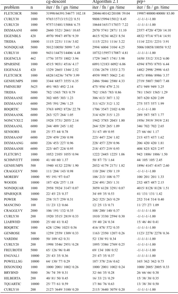
In this section, we compare the performance of the proposed methods with those of the PRP+ method developed by Gilbert and Nocedal [10], and the CG_DESCENT method proposed by Hager and Zhang [11].
The PRP+ code was obtained from Nocedal’s web page at http://www.ece. northwestern.edu/˜ nocedal/software.html, and the CG_DESCENT code from Hager’s web page at http://www.math.ufl.edu/˜ hager/. The PRP+ code is co-authored by Liu, Nocedal and Waltz, and the CG_DESCENT code is coau-thored by Hager and Zhang. The test problems are unconstrained problems in the CUTE library [3].
We stop the iteration if the inequalitykg(xk)k∞≤10−6is satisfied. All codes were written in Fortran and run on PC with 2.66GHz CPU processor and 1GB RAM memory and Linux operation system. Tables 1 and 2 list all numerical results. For convenience, we give the meanings of these methods in the tables.
there;
• “Algorithm 2.1” is Algorithm 2.1 withρ =1 and the same line search as “cg-descent”;
• “prp+” means the PRP+ method with the strong Wolfe line search pro-posed by Moré and Thuente [16].
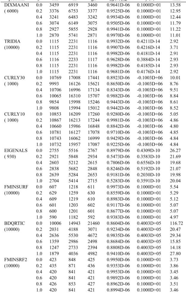
In order to get relatively betterρvalues in Algorithm 2.1, we choose 10 com-plex problems to test Algorithm 2.1 with differentρvalues. Table 1 lists these numerical results, where “problem”, “iter”, “fn”, “gn”, “time”, “kg(x)k∞” and “f(x)” mean the name of the test problem, the total number of iterations, the total number of function evaluations, the total number of gradient evaluations, the CPU time in seconds, the infinity norm of the final value of the gradient and the final value of the function at the final point, respectively.
In Table 1, we see that Algorithm 2.1 withρ =1 performed best. Moreover, we also compared Algorithm 2.1 with other Algorithms in the previous sections and numerical results showed that they performed similarly. So in this section, we only listed the numerical results for Algorithm 2.1 with ρ = 1, the “cg-descent” and “prp+” methods. These results are reported in Table 2 where “-1” means the method failed.
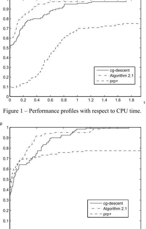
Figures 1–4 show the performance of the above methods relative to CPU time, the number of iterations, the number of function evaluations and the number of gradient evaluations, respectively, which were evaluated using the profiles of Dolan and Moré [7]. For example, the performance profiles with respect to CPU time means that for each method, we plot the fraction P of problems for which the method is within a factorτ of the best time. The left side of the figure gives the percentage of the test problems for which a method is the fastest; the right side gives the percentage of the test problems that are successfully solved by each of the methods. The top curve is the method that solved the most problems in a time that was within a factorτ of the best time.
0 0.2 0.4 0.6 0.8 1 1.2 1.4 1.6 1.8 0
0.1 0.2 0.3 0.4 0.5 0.6 0.7 0.8 0.9 1
τ p
cg-descent Algorithm 2.1 prp+
Figure 1 – Performance profiles with respect to CPU time.
0 0.5 1 1.5 2
0 0.1 0.2 0.3 0.4 0.5 0.6 0.7 0.8 0.9 1
τ p
cg-descent Algorithm 2.1 prp+
Figure 2 – Performance profiles with respect to the number of iterations.
0 0.2 0.4 0.6 0.8 1 1.2 1.4 1.6 1.8 0
0.1 0.2 0.3 0.4 0.5 0.6 0.7 0.8 0.9 1
τ p
cg-descent Algorithm 2.1 prp+
Figure 3 – Performance profiles with respect to the number of function evaluations.
0 0.5 1 1.5 2 2.5
0 0.1 0.2 0.3 0.4 0.5 0.6 0.7 0.8 0.9 1
τ p
cg-descent Algorithm 2.1 prp+
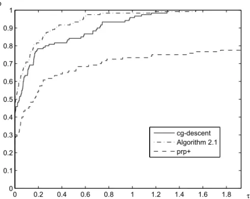
Figure 4 – Performance profiles with respect to the number of gradient evaluations.
6 Conclusions
searches. Moreover, we proved that the proposed HS methods converge glob-ally for strongly convex functions. Two modified schemes are introduced and proved to be globally convergent for general nonconvex functions. These results are also extended to some other conjugate gradient methods. Some results of the paper extend some work of the references [22, 23, 24]. The performance pro-files showed that the proposed methods are also efficient for problems from the CUTE library.
Acknowledgement. This work was supported by the NSF foundation (10701018) of China.
REFERENCES
[1] N. Andrei,Scaled conjugate gradient algorithms for unconstrained optimization. Comput. Optim. Appl.,38(2007), 401–416.
[2] E. Birgin and J.M. Martínez,A spectral conjugate gradient method for unconstrained opti-mization. Appl. Math. Optim.,43(2001), 117–128.
[3] K.E. Bongartz, A.R. Conn, N.I.M. Gould and P.L. Toint,CUTE: constrained and uncon-strained testing environments. ACM Trans. Math. Softw.,21(1995), 123–160.
[4] Y.H. Dai and L.Z. Liao,New conjugate conditions and related nonlinear conjugate gradi-ent methods. Appl. Math. Optim.,43(2001), 87–101.
[5] Y.H. Dai and Y. Yuan,A nonlinear conjugate gradient method with a strong global conver-gence property. SIAM J. Optim.,10(1999), 177–182.
[6] Y.H. Dai and Y. Yuan, Nonlinear Conjugate Gradient Methods. Shanghai Science and Technology Publisher, Shanghai (2000).
[7] E.D. Dolan and J.J. Moré,Benchmarking optimization software with performance profiles. Math. Program.,91(2002), 201–213.
[8] R. Fletcher and C. Reeves,Function minimization by conjugate gradients. Comput. J., 7(1964), 149–154.
[9] R. Fletcher,Practical Methods of Optimization, Vol I: Unconstrained Optimization. John Wiley & Sons, New York (1987).
[10] J.C. Gilbert and J. Nocedal,Global convergence properties of conjugate gradient methods for optimization. SIAM. J. Optim.,2(1992), 21–42.
[11] W.W. Hager and H. Zhang,A new conjugate gradient method with guaranteed descent and an efficient line search. SIAM J. Optim.,16(2005), 170–192.
[13] M.R. Hestenes and E.L. Stiefel,Methods of conjugate gradients for solving linear systems. J. Research Nat. Bur. Standards Section B,49(1952), 409–432.
[14] D. Li and M. Fukushima,A modified BFGS method and its global convergence in non-convex minimization. J. Comput. Appl. Math.,129(2001), 15–35.
[15] Y.L. Liu and C.S. Storey, Efficient generalized conjugate gradient algorithms, Part 1: Theory. J. Optim. Theory Appl.,69(1991), 129–137.
[16] J.J. Moré and D.J. Thuente,Line search algorithms with guaranted sufficient decrease. ACM Trans. Math. Softw.,20(1994), 286–307.
[17] B. Polak and G. Ribiere,Note sur la convergence des méthodes de directions conjuguées. Rev. Française Informat Recherche Operationelle,16(1969), 35–43.
[18] B.T. Polyak,The conjugate gradient method in extreme problems. USSR Comp. Math. Math. Phys.,9(1969), 94–112.
[19] D.F. Shanno,Conjugate gradient methods with inexact searches. Math. Oper. Res.,3(1978), 244–256.
[20] P. Wolfe,Convergence conditions for ascent methods. SIAM Rev.,11(1969), 226–235. [21] Y. Yuan and J. Stoer,A subspace study on conjugate algorithms. ZAMM Z. Angew. Math.
Mech.,75(1995), 69–77.
[22] L. Zhang, W. Zhou and D. Li,A descent modified Polak-Ribière-Polyak conjugate gradi-ent method and its global convergence. IMA J. Numer. Anal.,26(2006), 629–640. [23] L. Zhang, W. Zhou and D. Li,Global convergence of a modified Fletcher-Reeves
conju-gate gradient method with Armijo-type line search. Numer. Math.,104(2006), 561–572. [24] L. Zhang, W. Zhou and D. Li,Some descent three-term conjugate gradient methods and
their global convergence. Optim. Methods Softw.,22(2007), 697–711.