DOI: 10.1590/1808-057x201704320
Executive branch federal civil servant mortality by sex and
educational level – 1993/2014
Kaizo Iwakami Beltrão
Fundação Getúlio Vargas, Escola Brasileira de Administração Pública e de Empresas, Rio de Janeiro, RJ, Brazil
Sonoe Sugahara
Instituto Brasileiro de Geograia e Estatística, Escola Nacional de Ciências Estatísticas, Rio de Janeiro, RJ, Brazil
Received on 09.18.2016 – Desk acceptance on 10.04.2016 – 3rd version approved on 05.26.2017
ABSTRACT
Life tables have been elaborated throughout much of human history. However, the irst life table to use actuarial concepts was only constructed in 1815 by Milne for the city of Carlisle in England. Since then, numerous tables have been elaborated for diferent regions and countries, due to their crucial importance for analyzing various types of problems covering a vast range of possibilities, from actuarial studies to forecasting and evaluating demands in order to deine public policies. he most common problem nowadays in an actuarial calculation is choosing a suitable table for a given population. Brazil has few speciic tables for the pensions market and has been using imported tables that refer to other countries, with diferent cultures and diferent mortality experiences. Using data from the Integrated Human Resource Administration System, this table constructs life tables for Executive branch federal civil servants for the period from 1993 to 2014, disaggregated for sex, age, and educational level (high school and university). he international literature has recognized diferences in mortality due to sex, socioeconomic diferences, and occupation. he creation of the Complementary Pension Foundation for Federal Public Servants in 2013 requires speciic mortality tables for this population to support actuarial studies, healthcare, and personnel policies. A mathematical equation is itted to the data. his equation can be broken down into infant mortality (not present in the data), mortality from external causes, and mortality from senescence. Recent results acknowledging an upper limit for old age mortality are incorporated into the adjusted probabilities of death. Assuming a binomial distribution for deaths, the deviance was used as a igure of merit to evaluate the goodness of it of the observed data both to a set of tables used by the insurance/pensions market and to the adjusted tables.
1. INTRODUCTION
Life tables have been elaborated throughout much of human history. However, the irst life table to use strictly actuarial concepts was constructed in 1815 by Milne for the city of Carlisle in England. Since then, numerous tables have been elaborated for diferent regions and countries, due to their crucial importance for analyzing diferent types of problems covering a vast range of possibilities, from actuarial studies (Caldart, 2014) to forecasting and evaluating demands in order to deine public policies. he most common problem nowadays in actuarial calculations is choosing a suitable table for a given population. he creation of the Complementary Pensions Foundation for Federal Public Servants (Funpresp) in 2013 requires speciic mortality tables for this population to support actuarial studies, healthcare, and personnel policies.
Constructing a speciic life table for a population group presents two problems. he irst is the dataset in itself, containing information on deaths and the population at risk. Here it is possible to use cohort or cross-sectional data. he advantage of using cohort data lies in being able to observe the mortality rates of a single group at diferent ages. he disadvantage is the time needed to gather this data, as it is necessary to wait a whole generation from the birth to the death of the last member. With cross-sectional data, the data gathering time is reduced, but they observe deaths among diferent generations at diferent ages. he usual way is to construct what is called a synthetic cohort, using hypothetical individuals that would be exposed, at each age, to the force of mortality at a given time.
he second problem involves choosing a suitable model to describe some mortality function. Deaths can be considered as random variables with a binomial distribution, B(N,q), with the size parameter, N, being known (population exposed to risk) and the probability parameter, q, being unknown and still to be estimated. It is common to work with non-parametric models, in which the functions for the table for each age (or age group) are directly estimated from the data. Assuming that contiguous age groups (or contiguous ages) should present similar values for the functions, some type of smoothing considering the ages is usual. For this, various graduation techniques have been developed. Copas and Haberman (1983) divide the graduation methods into three main groups: graphical methods, parametric methods, and sum and adjusted means methods. Abid, Kamhawey, and Alsalloum (2006) divide the graduation actuarial methods into nine main blocks: graphical method, summation method, Kernel’s method, the method of
osculatory interpolation, the spline method, the curve itting or parametric method, graduation by reference to a standard table, diference equation method and linear programming method. On the other hand, each one of these approaches can incorporate time series variations or consider a particular point in time; that is, referring to a particular date.
he United Nations has created families of model tables, grouping those with similar characteristics (United Nations, 1983). here are four families (North, South, East, and West) indexed by a parameter. Although these tables have been created based on observation of 158 life tables, the indexation by a single parameter makes their use relatively limited. In contrast, there has been an extensive ofering of lexible parametric models to describe the forces of mortality for diferent ages. Some models aim to describe only adult mortality or some speciic age group. he irst more simplistic models assumed a maximum age and the functions that described the monitoring
of the cohort data were of the type: , in
which x is age, M is the maximum achievable age for the population, and nis an adjustment constant to be determined for the speciic population [see, for example, de Moivre (1718) and de Graaf (1729) cited by Duchene and Wunsch (1988)].
Gompertz (1825) proposes a model that, besides the random mortality that would afect young and old in the same way, adds a force of mortality related with senescence. here is no hypothesis for maximum lifespan. he resulting formula is:
in which x is age and the other parameters are constant in the equation and are still to be estimated.
Also in the same century, various authors proposed generalizations of this formula, mainly trying to better it extreme ages (the youngest and oldest). he proposed models based on the Gompertz formula were made more and more complex, although in the end none of them was completely satisfactory.
Other authors used various principles to formulate laws of mortality, for example using the Weibull distribution. In such cases, these authors (Morlat, 1975, cited by Duchene and Wunsch, 1988) assume that individuals are a composition of multiple and complex dynamic systems that interact with each other, each one with a Weibull
distribution with a speciic parameter. he combination of the various Weibull distributions has the same probability distribution. In this distribution, the force of mortality decreases with age like a hyperbola, while the Gompertz function assumes a constant force of mortality. he next stage was to propose models in which the mortality of each age group (or group of causes) presented a speciic behavior, and therefore had to be described by a diferent equation.
Obviously, the level and structure of mortality vary from population to population, and even in a speciic population, they vary in time. Studies on mortality rates have been developed considering the inluence of economic factors such as wealth. However, due to the diiculty of measuring this variable, it is common to use another variable that is highly correlated with income, such as education or occupation, which are more easily measured [see Vallin (1980)]. Masters, Hummer, and Powers (2012) explain the persistence of the importance of diferent educational levels for mortality, both for causes and for the aggregate.
Another aspect regarding mortality tables disaggregated by professional categories is common in developed countries. For example, in Great Britain statistics have been collected and published for more than 100 years, classifying workers into ive socioeconomic groups: Professionals, Managerial & technical intermediate, Skilled non-manual, Skilled manual, Partly skilled, and Unskilled. Some countries develop speciic mortality tables for the civil servant population (Andreone, 2011; Canada, 2014; Daric, 1951).
hese studies have also been carried out for mortalities from speciic causes. For example, Terris (1967) studied deaths from liver cirrhosis among diferent occupational groups in the United States of America and in other countries during the 1950s. Among his indings, Terris concluded that among 20- to 60-year-old men, manual workers (except those in agriculture) and those who were semi-qualiied had high mortality levels, of 48% and 18% above the American average, respectively. In contrast, during the same period in England and Wales it was observed that those groups with a higher educational level had twice as much chance of dying from cirrhosis than the less educated. he diference between these countries is attributable to the legislation for taxation. Alcoholic drinks are more heavily taxed in the countries mentioned than in the United States of America.
he main obstacle to constructing a life table using Civil Registry data (for information on deaths) and Censuses (for the population at risk) in Brazil and in other countries in a similar situation lies both in the level
of coverage of deaths and in the coverage and quality of the census information, although it is possible to estimate a corrector that uses any one of the various techniques that exist for estimating the levels of death coverage of the civil registry (Bennett & Horiuchi, 1981; Brass, 1975; Courbage & Fargues, 1979; Preston, Coale, Trussel & Weinstein, 1980). hese techniques assume a uniform error for all ages, or at least for the age groups above a certain age (usually 5 or 10 years). here is, however, evidence that these errors would be greater for the extreme groups: children and the elderly. Another problem is the use of data from diferent sources and possibly with diferent measurement and coverage errors. In Brazil, the problem of digit preference is notorious. It is common for people, especially the most elderly and those from a lower socioeconomic level, to state their age or year of birth by rounding the numbers to values ending in 0 or 5.
In this study, using the data from Siape, probabilities of death for active and retired Executive branch federal civil servants were estimated, extending the work of Beltrão and Sugahara (2002) and Borges (2009) and incorporating an expanded database to include 10 more years, thus obtaining more accurate estimates. hese estimates contribute to forming a set of mortality tables with experiences based on national data, and speciically,
they could support studies regarding public policies involving federal civil servants.
his article is composed of four sections. he irst is this introduction. he second describes and presents the development of the study and the third section includes the comments and conclusions. he last section contains the bibliography used. he Annex presents the values of the estimated tables for sex and educational level.
2. DEVELOPMENT
his section describes the source of the data used and the variables considered in the study and traces a proile of the contingent and of the public servant deaths found in the Siape database and used in calculating the probabilities of death. It also presents an adjusted model and the estimated parameters, as well as comparing the estimated tables according to sex and educational level and comparing these estimated tables with those used by the market.
2.1 Data source
With the reform of the State that started in 1995 (Brazil, 1995) and as part of a proposal for “reconstruction of the public administration on modern and rational foundations”, various information systems were developed to help in government management. Among these systems, a single system was created for the whole civil service in order to manage payroll and keep records on federal civil servants (Siape).
he system contains various iles organized into tables with various types of records, in which the civil servant’s registration is key for concatenation of the same records in the diferent tables. In volume, in December 2014 the Siape archive, the reference database for the data in this study, was composed of 1,447,670 observations corresponding to active, retired, and deceased federal civil servants. At the same time, the personnel list contained 1,207,106 active and retired workers and pension providers. Using the Siape personnel database,
a summarized ile was generated, containing, for each one of the registration records (including active, retired, and deceased employees, whether these were pension generators or not – information not provided), relevant information such as sex, age, educational level, and entity.
Some variables were chosen from those in the archive to use in this study. Some other variables were created using the information available. As an administrative record, Siape presents the advantages of working with a single source. hus, the numerator and the denominator of the probabilities of death are derived from the same source, as well as there not being the problem of under-registration or digit preference.
2.2 Distribution of the Federal Civil Servants
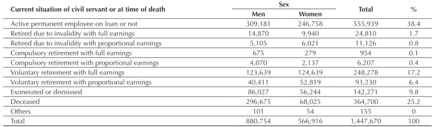
Table 1 Classiication of Executive branch federal civil servants in the register in December 2014, by sex and situation
Current situation of civil servant or at time of death Sex Total %
Men Women
Active permanent employee on loan or not 309,181 246,758 555,939 38.4
Retired due to invalidity with full earnings 14,870 9,940 24,810 1.7
Retired due to invalidity with proportional earnings 5,105 6,021 11,126 0.8
Compulsory retirement with full earnings 675 279 954 0.1
Compulsory retirement with proportional earnings 4,070 2,137 6,207 0.4
Voluntary retirement with full earnings 123,639 124,639 248,278 17.2
Voluntary retirement with proportional earnings 40,411 52,819 93,230 6.4
Exonerated or dismissed 86,027 56,244 142,271 9.8
Deceased 296,675 68,025 364,700 25.2
Others 101 54 155 0
Total 880,754 566,916 1,447,670 100
Source: Elaborated by the authors using data from the Integrated Human Resource Administration System (Siape).
Table 2 Classiicationof the Executive branch federal civil servants in the register in December 2014, by sex and educational level
Educational level Sex Total %
Men Women
0 13,522 1,117 14,639 1
Illiterate 8,685 1,061 9,746 0.7
Literate with standard courses 72,218 11,099 83,317 5.8
First level incomplete up to 4th grade incomplete 37 0 37 0
4th grade of irst level complete 190 63 253 0
Elementary school incomplete 108,102 27,840 135,942 9.4
Elementary school 92,106 47,365 139,471 9.6
Second level incomplete 110 47 157 0
High school 194,202 158,348 352,550 24.4
University incomplete 1,370 792 2,162 0.1
Middle level 477,020 246,615 723,635 51
University 374,412 305,812 680,224 47
Master’s 8,880 7,993 16,873 1.2
Doctorate 6,920 5,379 12,299 0.8
Higher level 390,212 319,184 709,396 49
Total 880,754 566,916 1,447,670 100
Source: Elaborated by the authors using data from the Integrated Human Resource Administration System (Siape). he values in Table 2 were obtained by classifying the
population of federal civil servants by educational level and sex. As already mentioned, the literature indicates diferent mortalities for educational level and sex. In this text, the decision was to group the employees into two more or
less equal sized groups: “higher level”, corresponding to those having completed higher education, a master’s, or doctorate, and “middle level”, including all educational levels below.
Following the proposed disaggregation of the population analysis into two main groups according to educational level, the information with this disaggregation is presented in Figure 1. he male (in blue) middle level population (let hand side pyramid) corresponds to a little more than six million person-years, while the female (in red) population is a little more than four million. For the men, the mode is presented as the threshold with very close values between 50 and 65 years, while for the women a single mode is discernable at 50 years. he
Figure 1 Sex/age distribution – population of active and retired civil servants – 1993/2014
Source: Elaborated by the authors using the data from the Integrated Human Resource Administration System (Siape).
Figure 2 presents, for the aggregate data between 1993 and 2014, the age pyramid of deaths in the active and retired population. he total deaths for those from the middle level (let hand side pyramid) is in the order of 173 thousand for men (in blue) and 47 thousand for women (in red). he proile of deaths for both sexes is unimodal, with the maximum at around 72 years for men
and 78 for women. As for the higher level population (right hand side pyramid), total deaths are almost 46 thousand for men and 14.4 thousand for women. For this higher level population, the proile of deaths is also unimodal, with the mode at around 72 and 73, for men and women, respectively.
150000 100000 50000 0 50000 100000 150000
20 30 40 50 60 70 80 90 100
MIDDLE LEVEL
Men Women
150000 100000 50000 0 50000 100000 150000
20 30 40 50 60 70 80 90 100
HIGHER LEVEL
Figure 2 Sex/age distribution – active and retired civil servant deaths – 1993/2014
Source: Elaborated by the authors using the data from the Integrated Human Resource Administration System (Siape).
2.3 Model Used
he following variables were used: px,s,e,t, for population of active and retired individuals with age x, sex s and educational level e (mean for year t) (population at risk), and dx,s,e,t, for deaths of the population of active and retired individuals occurring with age x, sex s and educational
level e (in year t). hese two variables were already described in the previous section and the aggregate data can be viewed in Figure 2 for the deaths and in Figure 1 for the population at risk. For the study, the years t = 1993 to 2014 were considered. he probabilities of death by sex, age, and educational level were initially calculated using the following formula, without any correction:
7000 6000 5000 4000 3000 2000 1000 0 1000 2000
20 30 40 50 60 70 80 90 100
MIDDLE LEVEL
Men Women
1600 1400 1200 1000 800 600 400 200 0 200 400 600
20 30 40 50 60 70 80 90 100
HIGHER LEVEL
in which q(x,s,e,t) is the probability of death of an individual from the population, with age x, sex s, and educational level e (in year t); px,s,e,t is the population exposed to risk (of active and retired individuals) with age x, sex s and educational level e (approximated as the mean of the population at the beginning and at the end of year t). By hypothesis, inlows and outlows not through deaths are considered as uniform over the year; dx,s,e,t are the deaths for the population of active and retired individuals occurring with age x, sex s and educational level e (in year t). By hypothesis, deaths are also considered uniform over the year. In the case of a closed population, the denominator is reduced to the population at the beginning of the year and the distribution of deaths is exactly a binomial. With inlows and outlows occurring through exoneration and new hirings over the year (always small lows in comparison to the population), this distribution is approximated. he Poisson distribution could be used as an approximation of the binomial distribution if the product of the exposed population size and of the probability of death was a
small value and the size of the population was large. In this study, this approximation is not advisable, due to the populations at the advanced ages being very sparse and the probabilities of death not being small.
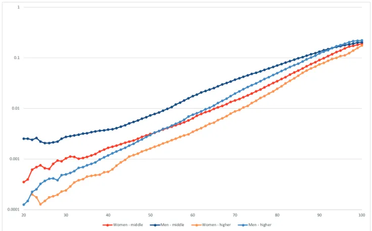
Figure 3 shows the probability of death according to sex, age, and educational level estimated for the period 1993/2014. Typically, men present higher values than women and individuals from the middle level present higher values than their higher level counterparts. In particular, the probability for the population of Men – middle level (dark blue line) is the highest, but with a possible cross-over in the upper ages with the probabilities of the higher level male population (light blue line). he probabilities of death of the middle level women (red line) lie, for the young adults (less than 40 years), in second place, directly below the probabilities related to the middle level men. From around 50 years, they are overtaken by the probabilities of death among higher level men, which in the lower ages lie in third place. he probabilities for higher level women (orange line) are consistently below all of the others.
Figure 3 Probabilities of death according to sex, age, and educational level – active and retired civil servants – 1993/2014
Source: Elaborated by the authors using the data from the Integrated Human Resource Administration System (Siape).
2
� �
,
�
,
�
,
�
=
�
�,�,�,��
�,�,�,�+
�
�,�,�,�⁄
2
0.0001 0.001 0.01 0.1 1
20 30 40 50 60 70 80 90 100
he curves suggest that it would be possible to it a function to these possibilities.
he decision was taken to test the families of functions suggested by Heligman and Pollard (1980) and already
successfully used by Beltrão and Sugahara (2002, 2005), Borges (2009), Oliveira et al. (2012), and Silva (2010).
he full model, as proposed by Heligman and Pollard (1980), includes three components:
in which the irst term (with parameters A, B, and C) describes mortality in early childhood. Unfortunately, there is no information on mortality related to this segment for this population, and so this component cannot be itted and the adjusted mortality only refers to adult mortality (including the elderly up to 100 years). Probably, with information on most years it would be possible to improve the estimates for the elderly. Data for the irst component (using information on survivors’ pensions) are also unlikely to be available. he second term corresponds to mortality from external causes. Deaths from external causes correspond to chapter XX of the International Classiication of Diseases (Brazil, 2015). hese causes of mortality mainly afect the male population and in Brazil they are the main causes of deaths among young male adults. In the data, this cause
is only evident among the middle level male and female population. The D parameter is related to the level of the “bump”, while the E parameter is related to its amplitude and the F parameter is a location parameter, laterally shiting the curve in the ages and at the same time characterizing the mode of this component (equal to 1nF). he last term corresponds to mortality from senescence and enables a deceleration (or acceleration) of mortality to be itted to the individuals in old age. his term is what varies between the diferent families proposed by Heligman and Pollard (1980). he G parameter can be simply understood as a shit of (lnG) in the age scale. he H parameter regulates the changes in the curvatures, as all begin concave and become convex. he higher H, the earlier the inlexion occurs. he functional form of this term for another family considered by the authors is:
As the data for the eldest group are scarce, even though the it has been carried out for all ages up to 100 years, there is no intention for the estimated curves to be used above 90 years. As the itted probabilities present a cross-over between the sexes due to a fall in male mortality in
the ages above 92, for ages above 90 the female probability was chosen as a reference.
Eliminating the irst component, the family that best its the data was a sum of exponentials in the form:
for middle level men and women and
for higher level men and women (eliminating the irst two terms).
3
4
5
3. RESULTS
his section presents the it made and compares this with the selected tables used by the insurance and pensions market.
3.1 Fits for Probability of Death
he person-years and deaths for the period 1993/2014 were considered for the parameters D, E, F, G, H, and K for men and women, as well as for each one of the educational levels (parameters D, E, and F appear only for the middle level). he estimation was carried out iteratively, using the non-linear regression analysis tool from the Statistical Package for the Social Sciences (SPSS), deining weights for the records (analysis/regression/nonlinear). he deaths observations for a particular age, educational level, and
sex are assumed to be distributed as random binomial variables B (Nx,e,s, qx,e,s), in which Nx,e,s is the population of civil servants of a particular age x, educational level e, and sex s, adjusted for inlows, outlows, and deaths, all of which are assumed to be uniform over the year, and qx,e,s
is the probability of death which needs to be determined. he non-linear regression procedure of the SPSS package does not enable the choice of this distribution (in fact, it is only possible to directly obtain optimal estimators for the normal distribution). Iteratively, estimators were calculated using weights that were inversely proportional to the standard deviation of the binomial based on the estimators from the previous stage. In the i–th step the weight, weight x,e,s (i), was calculated based on the probability
of death estimated in the previous step, qx,e,s (i-1); that is:
For the irst step, the population for each age, sex, and educational level were used as a weight, equivalent to assuming that the probabilities are constant for all the ages. he convergence was always quick, with ive iterations at most. he stop criterion was obtaining a diference between successive estimates of the parameter lower than 10-10. he K parameter was tested and shown
to be statistically different from the unit for all the combinations of sex and educational level, with the exception of the population of higher level men. As this population was the only case, the decision was taken to maintain the parameter in the equation of the model for this combination. All the estimated parameters were statistically signiicant. For the middle level group, the ages between 20 and 100 (included) were used in the it. For the higher level group, the age interval used was between 25 and 100 (included).
As already mentioned, the inexistence of people working for the government in lower ages than the limits used does not allow the estimation of the irst component of the Heligman and Pollard model (1980), and consequently the mortality estimate for obtaining a complete table starting from age zero. One suggestion for ages below 20 (or 25) would be concatenation with tables from the Brazilian Institute for Geography and Statistics (Instituto Brasileiro de Geograia e Estatística – IBGE), using a logit transformation to guarantee continuity. For
the centenarians, although the data exists, they are very sparse and there are doubts about their reliability. here is no consensus among the specialists about what the curve related to centenarian ages should be like. here is conlicting evidence and the information is all highly dependent on the quality of the data (Caselli & Vallin, 2001; Duchene & Wunsch, 1988). he growth rate of mortality appears to slow down for the elderly, but the controversy is due to the cause. Simple facts, such as mixture of populations, each one with a speciic mortality curve, can imply a deceleration and even decrease in the mortality rate as a function of age for the aggregate population.
he discussion in the literature from the Society of Actuaries (SOA, 2001, 2014) with regards to the construction of the RP tables indicates a deceleration in mortality rates in advanced ages, resulting in a plateau with a below-unit value (Gampe, 2010; Gavrilov & Gavrilova, 2011; Kestenbaum & Ferguson, 2010, cited by SOA, 2014). In this text, the same limit for men and women was assumed, similar to that adopted by the SOA when developing the RP tables. Moreover, the same threshold was assumed for both educational levels: 0.5. To guarantee this limit, the adjusted probabilities for the ages above 90 were recalculated as a weighted mean between the adjusted value and the limit value, using the value (age-90)/30 as a weight. hat is, at 119 years, the value reaches almost 0.5 and the subsequent value is equaled to one unit.
Table 3 Estimated parameters of the curve adjusted for sex and educational level
Level D E F G H K
Women
Middle 0.00031 4.00 29.00 0.00004937 1.08447 -2.0807
Men 0.00236 2.60 18.00 0.00012529 1.08582 2.8139
Women
Higher - - - 0.00001629 1.09440 -3.1930
Men - - - 0.00002420 1.10061 0.9314
Source: Elaborated by the authors using the data from the Integrated Human Resource Administration System (Siape).
Considering that the differences for sex and for educational level are determinants for the mortality proile, in which each group follows a sex and educational level combination, it is analyzed separately; however the graphics are shown according to the civil servants’ educational level.
3.2 Comparison of the Results - Sex and Educational Level
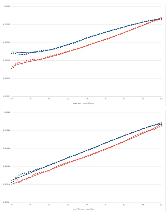
Figure 4 shows the comparisons of the results related to the adjustments of the chosen models (continuous lines) with the raw data (points) for men (in blue) and women (in red) from the middle (let hand side) and higher (right hand side) educational levels. For the ages below 40, for
Similarly to what was observed for middle level men, the negative K parameter for the higher level indicates mortality with decelerating growth in the higher ages. In the same way as was observed for middle level women, the positive K parameter for those from the higher level indicates mortality with accelerating growth in the higher ages, visible even for the ages below 100.
he male over-mortality is greater for the middle level
population and among the earlier ages, as expected. For the middle level population, the probability of male death is almost 7 times that for females at 20 years, falling with age until reaching the same level at 97. As for the higher level population, at 20 years, the over-mortality is a little below 2, rising slightly with age, reaching a maximum at 73 and falling ater this age, with a cross-over at 80 years with the over-mortality of the middle level population.
Figure 4 Probability of death according to age, sex, and educational level – active and retired civil servants – 1994/2013
Source: Elaborated by the authors using the data from the Integrated Human Resource Administration System (Siape).
0.00001 0.00010 0.00100 0.01000 0.10000 1.00000
20 30 40 50 60 70 80 90 100
Men Women
0.00001 0.00010 0.00100 0.01000 0.10000 1.00000
20 30 40 50 60 70 80 90 100
he over-mortality for educational level (probabilities of the middle level in the numerator and of the higher level in the denominator) is greater for the male population and in the earlier ages, as expected. For the male population, the probability of death for the middle level is almost 18 times that of the higher level at 20 years, falling with age until reaching the same levels immediately ater 90. his value, in the earlier ages, is mainly due to the diferent mortality from external causes, which is much greater for the population with the lower educational level. As for the female population, at 20 years, the over-mortality is a little above 4 (values for the middle level around four times the value for the higher level), falling with age and with a cross-over at 80 years with the over-mortality of the male population.
3.3 Comparison with Market Tables
This section presents the comparisons between the
estimated tables for the whole period, 1993/2014, for the four combinations of sex and educational level, with selected tables used by the insurance market [for characteristics of these tables, see SOA (2017)]. These comparisons are made based on the probabilities of death and a igure of merit, the deviance, which summarizes the quality of the it for all ages in one statistic.
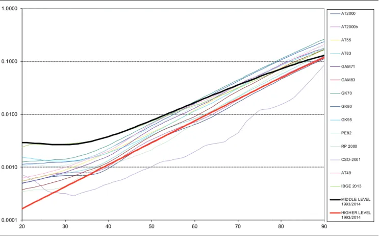
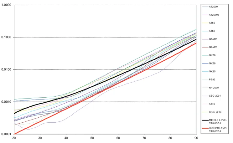
Figure 5 and Figure 6 present for men and women, respectively, the comparison of the estimated mortalities for the 1993/2014 period (reference January 2004, middle of the period) for civil servants according to educational level, and some selected life tables used by the insurance market. For men in the youngest ages, the estimated values for the civil servants almost serve as an upper (middle level) and lower (higher level) limit for the mortalities presented in the market tables. The exceptions are the upwards IBGE tables and the downwards Commissioner’s Standard Ordinary Tables(CSO, 2001). For women, the adjusted values appear in a much lower relative position.
Figure 5 Probability of death (log scale) – active and retired Executive branch federal civil servants according to educational level – men –1993/2014 – comparison of the adjusted values with market tables
Source: Elaborated by the authors using the data from the Integrated Human Resource Administration System (Siape).
0.0001 0.0010 0.0100 0.1000 1.0000
20 30 40 50 60 70 80 90
AT2000
AT2000b
AT55
AT83
GAM71
GAM83
GK70
GK80
GK95
PE82
RP 2000
CSO-2001
AT49
IBGE 2013
Figure 6 Probability of death (log scale) – active and retired Executive branch federal civil servants according to educational level – women –1993/2014 – comparison of the adjusted values with market tables
Source: Elaborated by the authors using the data from the Integrated Human Resource Administration System (Siape).
As can be observed, the goodness of it to the raw data of the diferent tables used by the market varies quite a lot with age and sex. It is worth remembering that the common practice in the case of private insurance companies is not to choose the table with the highest goodness of it, but to use one established by the market, assuming a loading factor (corresponding to a unilateral conidence interval) or a lateral shit in age, to guarantee the solvency and proitability of the system. For closed private pensions, a loading can be used for plans with smaller contingents, due to the variance associated with the process. For public schemes with higher contingents of personnel, the variance can be absorbed by the system, but in a payout system an adequate choice enables a better evaluation of future spending, as well as better planning of personnel policy.
The use of figures of merit that summarize the goodness of it of a dataset to a particular table (or set of tables) is common. In this text, the deviance (Croix, Planchet & Thérond, 2013; Dobson & Barnett, 2008) is used. It is deined as two times the diference between
the log likelihood of the saturated model and that of the table being tested; that is,
In the saturated model, the probabilities for each age coincide with the crude probabilities, . This statistic has an asymptotic distribution χ2 with the number of
degrees of freedom being equal to that of the individual ages used and it is derived from the likelihood ratio test. In this text, the statistics for the interval of ages between 30 and 80 were considered.
The literature mentions other igures of merit, some also based on the vraisemblance function, such as the Wald and the Score tests. These and the deviance are asymptotically equivalent, converging towards the same distribution χ2.
Considering that the distribution of deaths for a given age x and sex s follows, as already mentioned, a binomial distribution B [N(x,s);qtb(x,s)], in which N(x,s) is the population at risk with age x and sex s, assuming a given
table tb, with a speciic probability of mortality qtb(x,s) and with õ being the vector of observed deaths, the likelihood
of table Tb for a given sex s would be deined as:
0.0001 0.0010 0.0100 0.1000 1.0000
20 30 40 50 60 70 80 90
AT2000
AT2000b
AT55
AT83
GAM71
GAM83
GK70
GK80
GK95
PE82
RP 2000
CSO-2001
AT49
IBGE 2013
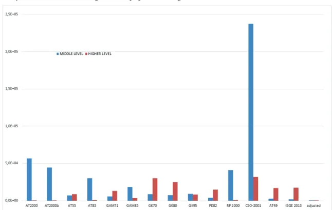
Figure 7 - Deviance of the selected and adjusted tables in relation to the raw values observed – active and retired Executive branch federal civil servants according to educational level – men –1993/2014
Source: Elaborated by the authors using the data from the Integrated Human Resource Administration System (Siape).
in which d(x,s) are the deaths occurring with age x and sex s and the corresponding log likelihood would be:
he deviance would then be:
Below, for each educational level, the graphics with the deviance values calculated for each combination of sex and table considered, are presented for analysis. he advantage of the deviance is that this igure of merit not only takes the statistical distribution of the data into account, but also the age proile of the population involved.
Figures 7 and 8 present the values for the deviances calculated for the 30- to 80-year-old age group for each sex, respectively, for the middle and higher level population
of Executive branch civil servants. It is noted that in the case of this igure of merit, the search is for the table that minimizes the value. Both for middle and for higher level men, the table with the best goodness of it, considering the deviance as a igure of merit, is the adjusted one and the worst is CSO-2001. In the case of higher level men, AT2000b is presented as a second alternative, with a deviance in the same order of magnitude of three times greater.
8
9
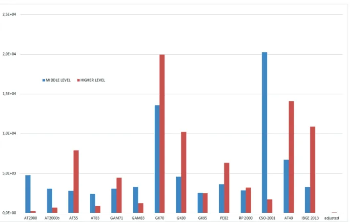
For the middle and higher level women, the tables with the best goodness of it are the adjusted tables, the same identiied for men. he table with the worst goodness of it for the middle level is CSO-2001, and for the higher level it
is GK70. For higher level women, table AT2000 is presented as a second option, with a deviance in the same order of magnitude as the adjusted table of ive times greater.
4. FINAL REMARKS
his study conirms the expected behavior of the mortality ranks. In theory, both sexes of the Brazilian population should present higher values than those of civil servants, both middle level and higher level. It is observed that the mortalities of higher level civil servants were lower than those of middle level civil servants, both for men and for women. his appears to indicate that the socioeconomic conditions associated with educational level also afect mortality among Brazilian civil servants, conirming similar studies carried out in other countries. This gap in socioeconomic conditions, which also translates into a gap in mortality, is smaller among women.
As was expected, the values obtained for women were always lower than the values found for men. Continuity of the study to estimate probabilities of death in other time intervals would be ideal. he monitoring of speciic
populations could work as a sentinel-event for larger populations, possibly signaling the existence of trends, such as the bump in mortality among young adults of both sexes, notable even with the scarcity of points in time among the middle level civil servants of both sexes.
Probabilities of death for the population as a whole depend, on one hand, on the availability of information on deaths from the IBGE Civil Registry or from the Ministry of Health’s Mortality Information System (SIM), which is not available in real time, as the administrative data of Siape is. On the other hand, they also depend on population information from the Census, which are usually collected at a ten-year time interval or from inter-census estimates. Probabilities calculated using the administrative records can be done in real time and with numerator and denominator information from the same source.
Figure 8 - Deviance of the selected and adjusted tables in relation to the raw values observed – active and retired Executive branch federal civil servants according to educational level – women –1993/2014
Moreover, specific life tables for a contingent of employees can be used to devise the institution’s policies. It is possible, for example, to estimate future spending on retirements and pensions. It is also possible to plan a future hiring scheme based on the outlows from the body of employees (whether through death, retirement, or exoneration). It is also possible to devise awareness campaigns for preventable causes of a greater magnitude in the group, such as, probably, external causes, cardiovascular diseases, etc.
One possible extension of this study would be a modeling that considers the improvement in the probabilities of death and a measure of their temporal variation (Rosner et al., 2013). One option for this extension could be a modiication of the model proposed by Lee and Carter (1992), considering the probabilities of the product of the model from Heligman and Pollard (1980) and a smooth deterministic function of age and time, instead of the random function, originally proposed by Lee and Carter.
REFERENCES
Abid, A. D., Kamhawey, A. A., & Alsalloum, O. I. (2006). Graduating the Saudi crude mortality rates and constricting their monetary tables. Journal of King Saud University, 19(1), 23-39.
Andreone, F. (2011). Le système de pensions des fonctionnaires et agents del’Union européenne. Revue Française D’administration Publique, 140(4). Retrieved from https://www.cairn.info/article_p.php?ID_ ARTICLE=RFAP_140_0807.
Beltrão, K. I., Sobral, A. P. B., Leal, A. A. C., Conceição, M. C. G. (1995, setembro). Mortalidade por sexo e idade dos funcionários do Banco do Brasil, 1940-1990. (Relatórios Técnicos, 02/95). Escola Nacional de Ciências Estatísticas/Instituto Brasileiro de Geograia e Estatística, Rio de Janeiro. Retrieved from http:// biblioteca.ibge.gov.br/visualizacao/livros/liv25525.pdf. Beltrão, K. I., Sugahara, S. (2002). Tábua de mortalidade
para os funcionários públicos civis federais do poder executivo por sexo e escolaridade: comparação com tábuas do mercado. (Texto para discussão, 3). Escola Nacional de Ciências Estatísticas/Instituto Brasileiro de Geograia e Estatística, Rio de Janeiro. Retrieved from http://biblioteca.ibge.gov.br/visualizacao/livros/ liv1419.pdf.
Beltrão, K. I., Sugahara, S. (2005). Taxas de mortalidade no setor de seguros – 1998/2000. Estimativas e comparações com tábuas de mercado: vida individual, vida em grupo, previdência privada e acidentes pessoais. (1a ed.). Rio de Janeiro: Fundação Escola Nacional de Seguros.
Bennett, N. G., & Horiuchi, S. (1981). Estimating the completeness of death registration in a closed population: current items. Population Index, 47(2), 207-222.
Borges, G. M. (2009). Funcionalismo público federal: construção e aplicação de tábuas biométricas.
(Dissertação de Mestrado). Escola Nacional de Ciências Estatísticas/Instituto Brasileiro de Geograia e Estatística, Rio de Janeiro. Retrieved from http:// www.ence.ibge.gov.br/images/ence/doc/mestrado/ dissertacoes/2009/Dissertacao_2009_Gabriel_ Mendes_Borges.pdf.
BRASIL. Ministério da Administração Federal e da Reforma do Estado (1995). Plano diretor da reforma
do aparelho do Estado. Brasília. Retrieved from http:// www.bresserpereira.org.br/Documents/MARE/ PlanoDiretor/planodiretor.pdf.
BRASIL. Ministério da Saúde. Classiicação estatística internacional de doenças e problemas relacionados à saúde – CID-10. Retrieved from http://www.datasus. gov.br/cid10/V2008/cid10.htm.
Brass, W. (1975). Methods for estimating fertility and mortality from limited and defective data. Chapel Hill: University of North Carolina, International program of Laboratories for Population Statistics.
Caldart, P., Motta, S., Caetano, M., & Bonatto, T. (2014). Adequação das hipóteses atuariais e modelo alternativo de capitalização para o regime básico do RPPS: o caso do Rio Grande do Sul. Revista Contabilidade & Finanças, 25(66), 281-293. Canada. Oice of the Superintendent of Financial
Institutions (2014). pension plan for the public service of Canada Mortality Study. Actuarial Study n. 14.
Ottawa: Oice of the Chief Actuary. Retrieved from http://www.osi-bsif.gc.ca/eng/docs/pscms.pdf. Caselli, G., & Vallin, J. (2001). Une demographie sans
limite? Population, 56(1), 51-83.
Conde, N. C. (1991). Tábua de mortalidade destinada a entidades fechadas de previdência privada (Dissertação de Mestrado). Ciências Contábeis e Atuariais, Pontifícia Universidade Católica de São Paulo, São Paulo.
Copas, J.B., & Haberman, M. A. (1983). Non-parametric graduation using kernel methods, Journal of the Institute of Actuaries, 110(1), 135-156.
Courbage, Y., & Fargues, P. (1979). A method for deriving mortality estimates from incomplete vital statistics.
Population Studies, 33(1), 165-180.
Croix, J.-C., Planchet, F., & hérond P.-E. (2013). Mortality: a statistical approach to detect model misspeciication. In Papers and Presentations of the Colloquium of the International Actuarial Association. Lyon. Retrieved from http://www.actuaries.org/ lyon2013/papers/LIFE_Croix_Planchet_herond.pdf. Daric, J. (1951). Mortality, occupation, and
Correspondence address:
Kaizo Iwakami Beltrão
Fundação Getúlio Vargas, Escola Brasileira de Administração Pública e de Empresas Rua Jornalista Orlando Dantas, 30, Sala 218 – CEP: 22231-010
Botafogo – Rio de Janeiro – RJ – Brasil Email: [email protected]
Dobson, A. J., & Barnett, A. (2008). An introduction to generalized linear models (3a ed.). London: Chapman and Hall/CRC.
Duchene, J., & Wunsch, G. (1988). Population aging and the limits to human life. Working paper 1. Bruxelles: Département de Démographie/Université Catholique de Louvain.
Gompertz, B. (1825). On the nature of the function expressive of the law of human mortality and on a new mode of determining life contingencies. Philosophical Transactions of the Royal Society,115, 513-585. Heligman, L., & Pollard, J. H. (1980). he age pattern
of mortality. Readings in Population Research Methodology, 2, 97-104.
Lee, R. D., & Carter, L. R. (1992). Modeling and forecasting the time series of US mortality. Journal of the American Statistical Association, 87(419), 659-671. Masters, R. K., Hummer, R. A., & Powers, D. A. (2012).
Educational diferences in U.S. adult mortality: a cohort perspective. American Sociological Review,
77(4), 548-572.
Oliveira, M., Frischtak, R., Ramirez, M., Beltrão, K., & Pinheiro, S. (2012). Tábuas biométricas de mortalidade e sobrevivência – experiência do mercado segurador brasileiro – 2010. Rio de Janeiro: Funenseg. Preston, S., Coale, A. J., Trussell, J., & Weinstein, M.
(1980). Estimating the completeness of reporting of adult deaths in populations that are approximately stable. Population Index, 46(2), 79-202.
Ribeiro, E. F., & Pires, V. R. R. (2001). Construção de tábua de mortalidade: experiência Banco do Brasil (Dissertação). Escola Nacional de Ciências
Estatísticas/Instituto Brasileiro de Geograia e Estatística, Rio de Janeiro.
Rosner B., Raham, C., Orduña, F., Chan, M., Xue, L., Benjazia, Z., & Yang, G. (2013). Literature review and assessment of mortality improvement rates in the U.S. population: past experience and future long-term trends. SOA. Retrieved from https://www.soa.org/iles/ research/exp-study/research-2013-lit-review.pdf. Silva, L. G. C. (2010, setembro). A tábua de mortalidade
do RPPS do estado de São Paulo. In Anais do XVII Encontro Nacional de Estudos Populacionais. Caxambu. Retrieved from http://www.abep.org.br/ publicacoes/index.php/anais/article/view/2293/2247. Society of Actuaries. (2001). he RP-2000 Mortality Tables.
Revised April 2001. Retrieved from https://www.soa. org/Files/Research/Exp-Study/rp00_mortalitytables. pdf.
Society of Actuaries. (2014). RP-2014 Mortality Tables Report. Revised November 2014. Retrieved from https://www.soa.org/Files/Research/Exp-Study/ research-2014-rp-report.pdf.
Society of Actuaries. (2017). Mortality and other rate tables. Retrieved from http://mort.soa.org/. Terris M. (1967). Epidemiology of cirrhosis of the liver:
national mortality data. American Journal of Public Health and the Nation’s Health, 57(12), 2076-2088. United Nations. (1983). Manual X: indirect techniques for
demographic estimation. New York: United Nation Publication.
Annex - Estimated values for the probabilities of death (qx)
Age Middle level women Middle level men Higher level women Higher level men
20 4.2851822E-04 2.9392781E-03 9.8993071E-05 1.6457956E-04
21 4.7554984E-04 2.9206961E-03 1.0834205E-04 1.8113487E-04
22 5.2256838E-04 2.8879381E-03 1.1857429E-04 1.9935519E-04
23 5.6902700E-04 2.8468176E-03 1.2977330E-04 2.1940792E-04
24 6.1457135E-04 2.8024574E-03 1.4203050E-04 2.4147725E-04
25 6.5904297E-04 2.7592656E-03 1.5544598E-04 2.6576590E-04
26 7.0246918E-04 2.7209667E-03 1.7012931E-04 2.9249693E-04
27 7.4504376E-04 2.6906640E-03 1.8620045E-04 3.2191578E-04
28 7.8710285E-04 2.6709203E-03 2.0379071E-04 3.5429255E-04
29 8.2909911E-04 2.6638434E-03 2.2304390E-04 3.8992445E-04
30 8.7157675E-04 2.6711714E-03 2.4411746E-04 4.2913848E-04
31 9.1514897E-04 2.6943529E-03 2.6718379E-04 4.7229446E-04
32 9.6047873E-04 2.7346194E-03 2.9243165E-04 5.1978829E-04
33 1.0082635E-03 2.7930500E-03 3.2006777E-04 5.7205555E-04
34 1.0592235E-03 2.8706270E-03 3.5031856E-04 6.2957545E-04
35 1.1140942E-03 2.9682842E-03 3.8343195E-04 6.9287521E-04
36 1.1736217E-03 3.0869482E-03 4.1967954E-04 7.6253483E-04
37 1.2385608E-03 3.2275727E-03 4.5935879E-04 8.3919235E-04
38 1.3096761E-03 3.3911687E-03 5.0279560E-04 9.2354960E-04
39 1.3877444E-03 3.5788291E-03 5.5034698E-04 1.0163786E-03
40 1.4735597E-03 3.7917507E-03 6.0240412E-04 1.1185284E-03
41 1.5679381E-03 4.0312528E-03 6.5939568E-04 1.2309328E-03
42 1.6717249E-03 4.2987938E-03 7.2179143E-04 1.3546188E-03
43 1.7858023E-03 4.5959862E-03 7.9010629E-04 1.4907158E-03
44 1.9110972E-03 4.9246100E-03 8.6490471E-04 1.6404653E-03
45 2.0485901E-03 5.2866255E-03 9.4680555E-04 1.8052325E-03
46 2.1993242E-03 5.6841857E-03 1.0364875E-03 1.9865182E-03
47 2.3644157E-03 6.1196479E-03 1.1346948E-03 2.1859719E-03
48 2.5450632E-03 6.5955849E-03 1.2422441E-03 2.4054065E-03
49 2.7425591E-03 7.1147971E-03 1.3600312E-03 2.6468142E-03
50 2.9583011E-03 7.6803229E-03 1.4890396E-03 2.9123839E-03
51 3.1938036E-03 8.2954507E-03 1.6303488E-03 3.2045199E-03
52 3.4507115E-03 8.9637291E-03 1.7851443E-03 3.5258630E-03
53 3.7308134E-03 9.6889782E-03 1.9547282E-03 3.8793130E-03
54 4.0360568E-03 1.0475299E-02 2.1405316E-03 4.2680533E-03
55 4.3685644E-03 1.1327086E-02 2.3441277E-03 4.6955777E-03
56 4.7306514E-03 1.2249030E-02 2.5672464E-03 5.1657197E-03
57 5.1248448E-03 1.3246131E-02 2.8117912E-03 5.6826842E-03
58 5.5539049E-03 1.4323705E-02 3.0798575E-03 6.2510817E-03
59 6.0208479E-03 1.5487382E-02 3.3737531E-03 6.8759658E-03
60 6.5289722E-03 1.6743112E-02 3.6960216E-03 7.5628733E-03
61 7.0818860E-03 1.8097166E-02 4.0494676E-03 8.3178677E-03
62 7.6835399E-03 1.9556124E-02 4.4371865E-03 9.1475857E-03
63 8.3382611E-03 2.1126872E-02 4.8625969E-03 1.0059288E-02
64 9.0507933E-03 2.2816584E-02 5.3294773E-03 1.1060911E-02
65 9.8263404E-03 2.4632705E-02 5.8420085E-03 1.2161128E-02
66 1.0670616E-02 2.6582921E-02 6.4048205E-03 1.3369404E-02
67 1.1589898E-02 2.8675128E-02 7.0230468E-03 1.4696068E-02
68 1.2591094E-02 3.0917387E-02 7.7023856E-03 1.6152373E-02
69 1.3681808E-02 3.3317872E-02 8.4491708E-03 1.7750572E-02
70 1.4870426E-02 3.5884811E-02 9.2704523E-03 1.9503988E-02
71 1.6166203E-02 3.8626410E-02 1.0174090E-02 2.1427092E-02
72 1.7579370E-02 4.1550772E-02 1.1168860E-02 2.3535582E-02
73 1.9121254E-02 4.4665798E-02 1.2264583E-02 2.5846458E-02
74 2.0804416E-02 4.7979081E-02 1.3472268E-02 2.8378098E-02
75 2.2642810E-02 5.1497787E-02 1.4804281E-02 3.1150339E-02
Age Middle level women Middle level men Higher level women Higher level men
77 2.6849207E-02 5.9177198E-02 1.7898812E-02 3.7503657E-02
78 2.9253897E-02 6.3348871E-02 1.9694869E-02 4.1132287E-02
79 3.1887737E-02 6.7747597E-02 2.1682954E-02 4.5096721E-02
80 3.4775110E-02 7.2376263E-02 2.3886125E-02 4.9424966E-02
81 3.7943488E-02 7.7236433E-02 2.6330760E-02 5.4146754E-02
82 4.1423928E-02 8.2328189E-02 2.9047152E-02 5.9293521E-02
83 4.5251646E-02 8.7649978E-02 3.2070249E-02 6.4898356E-02
84 4.9466731E-02 9.3198480E-02 3.5440559E-02 7.0995917E-02
85 5.4114986E-02 9.8968491E-02 3.9205280E-02 7.7622293E-02
86 5.9248978E-02 1.0495282E-01 4.3419721E-02 8.4814821E-02
87 6.4929303E-02 1.1114225E-01 4.8149103E-02 9.2611843E-02
88 7.1226173E-02 1.1752546E-01 5.3470861E-02 1.0105239E-01
89 7.8221377E-02 1.2408908E-01 5.9477637E-02 1.1017581E-01
90 8.6010761E-02 1.3081771E-01 6.6281180E-02 1.2002128E-01
91 9.4138035E-02 1.4062523E-01 7.3502933E-02 1.2911442E-01
92 1.0279240E-01 1.5086262E-01 8.1347383E-02 1.3874105E-01
93 1.1197774E-01 1.6151327E-01 8.9845480E-02 1.4890728E-01
94 1.2169681E-01 1.7256011E-01 9.9025870E-02 1.5961481E-01
95 1.3194931E-01 1.8398292E-01 1.0891408E-01 1.7086029E-01
96 1.4273184E-01 1.9575858E-01 1.1953166E-01 1.8263460E-01
97 1.5403795E-01 2.0786134E-01 1.3089523E-01 1.9492226E-01
98 1.6585823E-01 2.2026312E-01 1.4301553E-01 2.0770075E-01
99 1.7818041E-01 2.3293389E-01 1.5589646E-01 2.2094004E-01
100 1.9098964E-01 2.4584214E-01 1.6953414E-01 2.3460215E-01
101 2.0426869E-01 2.5895524E-01 1.8391600E-01 2.4864086E-01
102 2.1799831E-01 2.7223997E-01 1.9902003E-01 2.6300167E-01
103 2.3215747E-01 2.8566292E-01 2.1481417E-01 2.7762185E-01
104 2.4672381E-01 2.9919095E-01 2.3125585E-01 2.9243081E-01
105 2.6167394E-01 3.1279161E-01 2.4829182E-01 3.0735068E-01
106 2.7698383E-01 3.2643351E-01 2.6585821E-01 3.2229715E-01
107 2.9262916E-01 3.4008666E-01 2.8388088E-01 3.3718057E-01
108 3.0858566E-01 3.5372280E-01 3.0227615E-01 3.5190726E-01
109 3.2482941E-01 3.6731555E-01 3.2095173E-01 3.6638099E-01
110 3.4133713E-01 3.8084068E-01 3.3980799E-01 3.8050472E-01
111 3.5808643E-01 3.9427621E-01 3.5873953E-01 3.9418227E-01
112 3.7505602E-01 4.0760247E-01 3.7763687E-01 4.0732016E-01
113 3.9222583E-01 4.2080216E-01 3.9638832E-01 4.1982931E-01
114 4.0957723E-01 4.3386031E-01 4.1488196E-01 4.3162673E-01
115 4.2709303E-01 4.4676426E-01 4.3300753E-01 4.4263691E-01
116 4.4475758E-01 4.5950355E-01 4.5065839E-01 4.5279311E-01
117 4.6255681E-01 4.7206983E-01 4.6773313E-01 4.6203830E-01
118 4.8047819E-01 4.8445673E-01 4.8413719E-01 4.7032585E-01
119 4.9851072E-01 4.9665968E-01 4.9978406E-01 4.7761988E-01
120 1.0000000E+00 1.0000000E+00 1.0000000E+00 1.0000000E+00
Source: Elaborated by the authors using data from the Integrated Human Resource Administration System