1
MESTRADO
E
CONOMICS
TRABALHO FINAL DE MESTRADO
D
ISSERTAÇÃO
T
HE
R
OLE OF
G
OVERNMENT
D
EBT ON
E
CONOMIC
G
ROWTH
J
OSÉ
R
ICARDO
B
ORGES
A
LVES
2
MESTRADO EM
E
CONOMICS
TRABALHO FINAL DE MESTRADO
D
ISSERTAÇÃO
T
HE
R
OLE OF
G
OVERNMENT
D
EBT ON
E
CONOMIC
G
ROWTH
J
OSÉ
R
ICARDO
B
ORGES
A
LVES
O
RIENTAÇÃO:
A
NTÓNIOM
ANUELP
EDROA
FONSO1
José Ricardo Borges Alves
Supervisor: António Afonso Master in: Economics
Abstract
In our research, we study the effect of public debt on economic growth for annual and 5-year average growth rates, as well as the existence of non-linearity effects of debt on growth for 14 European countries since 1970 until 2012. We also consider debt-to-GDP ratio interactions with monetary, public finance, institutional and macroeconomic variables. We conclude that debt has a negative impact of -0.01% for each increment of 1% of public debt, although debt service has a 10 times worse effect on growth. We reach average thresholds for annual and 5-year average of 75% and 74%, respectively. Belonging to Eurozone has a detrimental effect of at least -0.5% for real per capita GDP, and banking crisis is the most harmful crisis for the growth phenomena.
JEL Codes: E62, H63, O47.
2
Acknowledgments
Firstly, I would like to thank to Professor António Afonso who gave me constantly support and motivation to proceed with my dissertation. The knowledge and the patient he had with me were crucial to handle all of this process. I am very proud to had Professor António Afonso as my supervisor.
I would also like to thank to ISEG-School of Economics and Management for providing me along this master course a theoretical and practical background which helped me to develop my social and intellectual skills. This thank is extended to all professors of ISEG, with who I had the most valuable life experience: the opportunity to learn and emancipate through the economic science.
I am very grateful to my parents and my brother Francisco, and to all of my friends for their support, technical help, constant motivation and intellectual discussions about my theme.
One last and very special thanks to Raquel Balhote for her comprehension, emotional and technical support and for understanding all my constant concerns during my work. I would thank to her all the friendship and love she gave me, even when I was troubled during some setbacks in this work.
3 Contents
1. Introduction ... 4
2. Literature Review ... 6
3. Methodology and Data ... 11
3.1. Analytical Framework... 11 3.2. Econometric approaches ... 12 3.2.1. Panel techniques ... 12 3.2.2. Heterogeneity ... 13 3.2.3. Endogeneity ... 14 3.2.4. Cross-sectional dependence ... 14 3.3. Data ... 15 4. Empirical Analysis ... 18 4.1. Debt-growth relationship ... 18
4.2. Non-linarities of government debt on growth ... 24
5. Conclusions ... 30
References ... 32
Appendix A – Data Statistics ... 37
Appendix B – Additional Results ... 39
4 1. Introduction
In 2007, a financial crisis emerged from the U.S. financial system, namely, from the banking sector with the bankruptcy of Lehman Brothers. As a result, the fiscal imbalances of several countries grew in a way that originated a sovereign debt crisis, beginning in Greece and crossing all Euro-area countries, especially, the peripheral countries such as Portugal, Italy, Ireland and Spain.
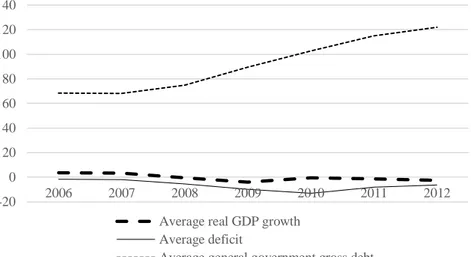
During 2006 and 2012, in these particular countries, the general government gross debt ratio increased, on average, from 68.36% to 121.94% of GDP, and the budget deficit ratio grew, on average and in absolute terms, from 1.59% to 6.48% of GDP. However, when comparing the evolution of real GDP in these countries, it is evident a decline in that same period: in 2006 the mean of the real GDP growth rate was 3.73%, decreasing to -2.48% in 2012. All this evolution can be observed in Figure 1.
Figure 1: Evolution of public finance variables in Portugal, Ireland Italy, Greece and Spain between 2006 and 2012.
-20 0 20 40 60 80 100 120 140 2006 2007 2008 2009 2010 2011 2012
Average real GDP growth Average deficit
Average general government gross debt
5
In addition to this economic performance, in 2010 a controversy aroused from the polemic Reinhart & Rogoff (2010) study about the effect of government debt on economic growth. Discussions regarding the evidence of mistakes in this paper fuelled the debate. Despite of economists and policymakers had focused their main debate in this central macroeconomics question, the economic and policy discussions have not being oriented yet, and in a precise way, for the real source of this problem. The multiple attempts taken by the governments until now just have prolonged the poor economic performance, along with several costs in general for the societies. Citing Buchanan (1966), the actual discussion around public debt has been a “murky battleground”. In his article, Buchanan places an important question which could be the main query posed by the social scientists and politicians: “Who pays, and when, for public expenditures that are financed by debt issue instead of taxation or money creation?”
Wright (1943) says even though “our problem, let me again repeat, is not: Can deficits someday roll up an intolerable debt? Our problem is: What are the maladjustments which are making continued deficits necessary? (…) Are the taxes too heavy or too light, or are they poorly distributed and levied?”
In contrast with this reality, economic theory tells us that government debt could be an important vehicle to induce economic growth, and this dissertation pretends assess this issue. Besides this interaction, we also want to study possible evidence of an inverted U-shape relationship between debt and growth. As our results show, debt has a detrimental effect on growth, although debt service represents a larger damaging consequence for growth. We find too, evidence of debt thresholds around 75% and 74% for annual and 5-year average growth rates, respectively.
6
The remaining part of this dissertation is organized as follows. Section two provides a literature review regarding the theoretical viewpoints and the empirical works on the effect of public debt on economic growth and their relationship with
monetary1, public finance, institutional and, lastly, macroeconomic variables. Section
three presents the methodology, several robustness tests, the data and its sources. Section four provides the empirical analysis. The last section presents the conclusions.
2. Literature Review
There is quite a lot of literature on economic theory about the importance of public debt on economic growth. Diamond (1965) describes a model that examines the long-run competitive equilibrium in a growth model and explores the effects of government debt on that same equilibrium. The author concludes that taxes have the same impact on individuals living during long-run equilibrium, whether they are used to finance internal or external debt. According to Feldstein (1985), in theoretical terms if the stock of capital is initially at an optimal level, it is better to finance a temporary increase in spending through debt because the excess burden of taxation depends on the square of the tax rate. When capital is below the optimal level, it is preferable to finance the amount of spending with taxation. These conclusions are taken from the relationship between capital intensity and the golden rule level: when capital intensity is less than the golden rule level, it implies that the government spending-labour force ratio is smaller than taxation per capita and so, the increase of debt must be financed by taxation.
1 In these results we will also show results regarding the - convergence process during the analysed
7
On the other hand, Martin (2009) tries to explain the level of debt affirming that the crucial determinant of this level is the compliance of households to substitute away goods being taxed by inflation. Despite of the welfare in an economy with debt being lower than an economy without debt, Wigger (2009) concludes that the generations could benefit from Ponzi schemes on issuing debt, depending on their preferences and on technology. Greiner (2012) relates a higher public debt ratio with a smaller long-run growth rate. However, in Greiner (2013), when the author assumes wage rigidity, the conclusion is different: public debt does not affect long-run economic growth or employment, only the stability of economy.
Focusing on empirical works about this subject, Schclarek (2004) investigates both linear and non-linear correlation among growth and government debt for developing and developed countries. For what matters in developed countries, the author does not find any linear or non-linear relationship between these two variables. Reinhart & Rogoff (2010) explore the possibility of a persistent relationship between high gross central government debt levels, economic growth and inflation based on a
new database2. The authors affirm the existence of a weak link between growth and low
levels of debt but when debt-to-GDP ratio is over 90%, the economies’ growth rates are on average one percent lower than otherwise.
While exploring the influence of high public debt on long-run growth, based on a panel data of advanced and developing countries over 38 years, Kumar & Jaejoon (2010) reach two important conclusions: an inverse relationship between initial debt and growth; and the possibility of some non-linearity effects of debt on growth. Afonso & Jalles (2013) analyse the linkages between growth, public debt and productivity
8
throughout the analysis of 155 countries between 1970 and 2008. The authors conclude that there is a negative effect of debt ratio and financial crisis on economic growth. Still, higher debt ratios could benefit Total Factor Productivity (TFP) growth. Reinhart & Rogoff (2011) compiled a database on domestic debt which allows a better comprehension about the query of why the economies default on external debts at low thresholds of public debt.
Another empirical work that helps understanding the role of public debt on economic growth is provided by Cecchetti et al. (2011) who analyse the debt damage effect for 18 OECD countries in a 30 years’ time span, reaching to an 85% government debt-to-GDP ratio threshold.
On the other hand, while investigating the same causality but now for twelve euro area countries between 1990 and 2010, Baum et al (2013) conclude there is a threshold rounding the 67% public debt ratio (above 95% there is a negative impact on economic growth) and the interest rates are pressured upward when debt ratio is greater than 70% of GDP. Checherita-Westphal & Rother (2012) study twelve euro-area countries since 1970 until 2010 and conclude that the negative effect of government debt on growth starts between 70% and 80%, and private saving, public investment and TFP are the channels whereby public debt is found to have a non-linear impact on growth. Introducing some political variables, Elgin & Uras (2012) relate the higher informal sector size with higher probability of sovereign default risk and country’s public indebtedness, for 155 countries using data from 1960 until 2008. Heylen, et al
(2013) analysing 132 fiscal episodes for 21 OECD countries over twenty-eight years
and reach to a conclusion: consolidation programs of public debt reduction are more successful when they are followed by product-market deregulation and when they are
9
adopted by left-wing governments. Labour market deregulation could have a contrary effect on debt reduction, as well as wage bill cuts (this last point is only effective when government efficiency is low).
Gnegne & Jawadi (2013) investigate public debt and its dynamics for the UK and USA, which proved to be asymmetric and nonlinear, conclude that public debt seems to be based on several threshold effects that help to understand, with more accuracy, its dynamics. Certainly, macroeconomic events such as economic slowdowns, debt and financial crisis, as well as oil shocks, are proved to be important factors linked with structural breaks in public debt dynamics. In Kourtellos et al. (2013), a structural threshold regression methodology is used to investigate the heterogeneity causalities of public debt on economic growth. Reviewing the effect of political variables, the authors highlight an evidence of an inverse relationship of democracy degree on threshold effects.
Revising on the existing literature about the sustainability of public finances, Westerlund & Prohl (2010) examine both public revenues and expenditures for eight OECD countries through a nonstationary panel data approach, in which the authors do not reject the sustainability hypothesis. Fincke & Greiner (2011) study the reaction of primary surplus (in percentage of GDP) to variations in debt to GDP ratio in some euro area countries. Considering the group of PIIGS countries, their results show that only Ireland, Portugal and Spain give the impression of following a sustainable debt policy. For Greece, the conclusion of a sustainable debt policy is rejected, while for Italy the results are slightly dubious. Using a Keynesian framework, Leão (2013) affirms that under the full employment level, a rise in public spending may diminish the level of public debt-ratio. Teica (2012), for instant, proposes an analysis of public debt
10
sustainability in the euro area countries and states that debt sustainability can be achieved throughout a mix of budgetary and fiscal policies in order to reduce budget deficits and increase primary balances.
Other articles, as Wahab (2004) and Kolluri & Wahab (2007), distinguish the relation between government expenditures in different periods of economic growth (in expansionary and in a recession movements) for OECD and euro area countries. The first one suggests an inverse relationship, namely the results indicate that public expenditures increase less than proportionately in a time of growth, and decrease proportionately more on a recession. The second article evidences the increase of government expenditure during periods of a negative economic growth, and it also highlights the Wagner’s proposition, which is less evident for euro-area members. On the other hand, in the Fölster & Henrekson (2001) article, the authors conclude that for all countries sample there is an evidence of both government expenditure and taxation being negatively related with growth.
In Campos, et al. (2006), the authors stress the importance of stock-flows reconciliation, that despite being commonly considered for many economists as a negligible entity to explain the dynamics of public debt growth, they found it as being a crucial determinant for debt dynamics. Contingent liabilities and balance-sheet effects, based on econometric tests done by the authors themselves, explain this variable. Gruber & Kamin (2012) examine the effect of the debt level and the fiscal balance for some OECD countries between 1988 and 2008, leading to a statistically significant impact of one percentage rise in the structural budget balance and net debt on the bond yield rates. Finally, Afonso & Jalles (2012), through a panel data of developed and emerging countries over 39 years, conclude a lesser economic growth in the presence of
11
increased fiscal policy volatility. Government spending presents symptoms of rigidity when compared with revenue during financial crisis periods.
3. Methodology and Data 3.1. Analytical Framework
This study uses the neoclassical growth model as the essential framework represented by the aggregate production function Y=F(K,L), where Y is the aggregate output, K is the capital stock (both human and physical) and L is the labour force or population. Admitting the hypothesis of heterogeneity across economies and therefore, the existence of different steady states, from the analysis of this production function the concept of convergence arises. According to Barro & Sala-i-Martin (2004), “an economy grows faster the further it is from its own steady-state value” or, in other words, the model expects that economies with a starting lower value of real per capita income tend to grow faster than economies with higher values of real income.
However, in this dissertation we will consider different variables, namely the government debt-to-GDP ratio, once there are other aspects that can explain the convergence phenomena, besides considering only the initial per capita income. The aggregate production is now F=(K,L,D), being D the debt-to-GDP ratio variable, which can be represented by the following equation:
(1) g y x Dit t i it t T i N j it i it it it 0 01 2 , 1,..., ; 1,..., ,
where g represents the real per capita GDP growth rate; it y the real per capita it
income of 1970, the initial year of our time-span analysed; j
it
x , j=1,2 is a vector of
12
respectively, the time effect and the country-specific effect; it is an unobserved zero
mean white noise-type column vector satisfying the standard assumptions;,0,1and
2
are unknown coefficients to be estimated.In order to study the non-linearity effect of government debt on economic growth, we will subsequently add to equation (1) the squared debt-to-GDP variable:
(2) g y xj Dit Dit t i it t T i N it i it it it , 1,..., ; 1,..., 2 3 2 1 0 0 .
Moreover, we will add several variables described in section 3.3 in order to determine the effect of debt-to-GDP ratio in real per capita income while interacting with the mentioned variables.
3.2. Econometric approaches 3.2.1. Panel techniques
Instead of using cross-section methods to analyse the public debt effects on growth, we use panel data techniques to compute those dynamics on real per capita growth. One of the important advantages on using panel data estimation is to highlight the individual heterogeneity, once there are some differentiating features across cross section. Those particularities could, or not, be constant across time, in a way that time series or cross-sectional approaches may not take into account that referred heterogeneity leading to biased results. Amongst other advantages we can name in data panel techniques, the ones we find more important, especially to our study, are: a largest data set available, which allows identifying and measure with more accuracy the individual effects of the sample, contrarily to cross-section and time-series methods; less colinearity; and a greater efficiency in obtaining the estimation results.
13
On the other hand, we should also stress some problems related with panel data approaches, such as the possibility of an impact caused by unobserved heterogeneity,
the lack of some particular data,3 biased estimators due to incorrect specification of the
model. Nevertheless, we should especially take into account problems related with endogeneity and cross-section dependence.
3.2.2. Heterogeneity
To deal with unobserved effects presented in equation (1), it is possible to apply a fixed effects or a random effects model. Admitting the existence of omitted variables and with the assumption of no correlation between the explanatory variables and the unobserved variables, the best way to handle with unobserved effects is using a random effects model. On the other hand, if the omitted variables and the explanatory variables are correlated, it is, then, preferred to apply a fixed effects model in order to deal with omitted variable bias.
Therefore, we apply the Hausman test to choose the best methodology to solve the problem of unobserved effects. The basic idea of this test is to examine if we can accept the null hypothesis, meaning that the random effects is the best solution, against its rejection, which concludes for the use of a fixed effects estimation. Through the Hausman test, the null hypothesis is rejected and so, we shall use the fixed effects
estimation.4
3 There are some variables for which there are no data available for some countries in particular years. 4 For reasons of parsimony, the results for this test are not presented here. However, they are available in
14 3.2.3. Endogeneity
As we mentioned earlier, the endogeneity problem is one of the main issues that can arise from panel data analysis. Once it could be present in regressors, one of the main objectives is to solve this problem in order to obtain unbiased estimators.
Endogeneity can emerge from omitted variables, measurement errors or simultaneity. This problem could lead to a rejection of “type 1 errors” or cause a failure when we pretend to reject the null hypothesis. Once the country-specific properties may carry on some unobserved omitted variables, for instance, by the misspecification of the model and with the natural consequence in obtaining biased estimators, that specific effect will not solve the endogeineity potential problem.
The Two Stage Least Squares estimator (2SLS) allows the correction of this problem of endogeneity, even for multiple endogenous explanatory variables. According to Wooldridge (2009), it is necessary to make use of order condition because when there is more than one endogenous variable, this could lead to a failure in the identification of the endogenous explanatory variable of our model. This referred condition uses the White diagonal covariance matrix in order to assume a residual heteroskedasticity.
3.2.4. Cross-sectional dependence
Sarafidis & Wansbeek (2010) mention that “one major issue that inherently arises in every panel data study with potential implications on parameter estimation and inference is the possibility that the individual units are interdependent.” The presence of cross-sectional dependence causes misspecification of the model once the explanatory variables can be correlated with shocks or unspecified variables. The authors propose
15
several methods to solve this problem for the weak and strong cross-sectional dependence such as, the LM statistic test, also proposed by Breusch & Pagan, (1980). When N is large, LM statistic presents “poor size properties”, citing the first authors’ article. Taking into account the nature of our study – the number of variables, years and countries – it will be discarded the use of this statistical methodology.
According to Chudik, et al. (2009), the common correlated effects (CCE) estimator, studied by Pesaran (2006), allows the estimations to remain consistent and it also allows the asymptotic normal theory to still be applicable for a large number of weak and semi-weak factors in panel data studies. Therefore, it is used the Pesaran’s CD test statistic in all of the methods used in the estimation. Lastly, we use the Generalized Least Squares (GLS) methodology to deal with cross-sectional dependence. As we will observe later in all the obtained results from econometric tests, we conclude that there is no cross-section dependence phenomenon, once the values computed for Pesaran’s CD test statistic rejects this hypothesis.
3.3. Data
The model is estimated for a period between 1970 and 2012 and for 14 European countries: Austria (AT), Belgium (BE), Denmark (DK), Finland (FI), France (FR), Germany (DE), Greece (GR), Ireland (IE), Italy (IT), the Netherlands (NL), Portugal (PT), Spain (ES), Sweden (SE) and United Kingdom (UK). The dataset excludes some euro-area and OECD countries with poor data availability, in order to avoid a large measurement error.
16
The database5 was collected from several sources. Real GDP (RGDP) per capita
and Real GDP growth rate (RGDPGR), urbanization rate (URB), domestic credit to private credit sector in percentage of GDP (CREDIT), inflation as the percentage change in the cost of average consumer of acquiring a basket of goods and services (INFLATION) and trade openness throughout the sum of exports and imports of goods and services in percentage of GDP (TRADEOPE) were retrieved from the World
Bank’s World Development Indicators.6 From AMECO database we collected the
following variables: general government gross debt in percentage of GDP at market prices (DEBT), nominal short-term interest rate (SHORTINT), cyclically adjusted primary balance (CAPB), output gap relatively to potential GDP at market prices (OUTPUTGAP), general government total expenditures (EXP), primary budget balance (PBB), total budget balance (TBB), and debt service (DEBTS), which was constructed through the subtraction between primary budget balance and the total budget balance.
Population levels in thousands (POP), gross fixed capital formation growth rate (GFCF), average hours actually worked (AVH), annual growth rate, in percentage, of unit labour costs in total economy (ULC), the annual growth rate of labour compensation per unit of labour input in total economy (LC), current account balance as a percentage of GDP (CURRENT), long-term interest rates (LONGINT), rate of unemployment in percentage of total labour force (UNEM), taxes on goods and services as percentage of GDP (TGOODS), taxes on income and profits in percentage of
5 The database used in this study is available in the following website: https://aquila2.iseg.ulisboa.pt/a
quila/homepage/l37655/base-de-dados---tfm.-the-role-of-government-debt-on-economic-growth
6 This dataset is available in the following website:
17
GDP (TINC), as well as life expectancy at birth, measured in number of years (LE),
were taken from OECD.7
From Beck, et al (2009)8, the liquid liabilities in percentage of GDP (M3), was
used. Other variables, such as the index of human capital per person (HC), capital stock at constant 2005 national prices (K), total factor productivity at constant national prices
(TFP), were based in Feenstra et al. (2013).9
In addition, we also use dummy variables. From Reinhart & Rogoff (2009)10
database, we consider banking crises (BANKINGC), currency crises (CURRENCYC), inflation crises (INFLATIONC) and stock market crash (STOCKMARKETC) as dummies that take the value “1” for the specific year when the referred crises happen). Another variable from the same source we take into account is crises tally (CRISESTALLY), which represents the sum of each crisis in a particular year. Lastly, applying the criteria of (Afonso, 2005), we built a euro-zone (EURO), Maastricht Treaty (MAAS) and Stability and Growth Pact (SGP) dummies (the variable takes the value “1”, if for each year the country is covered by such event). The descriptive
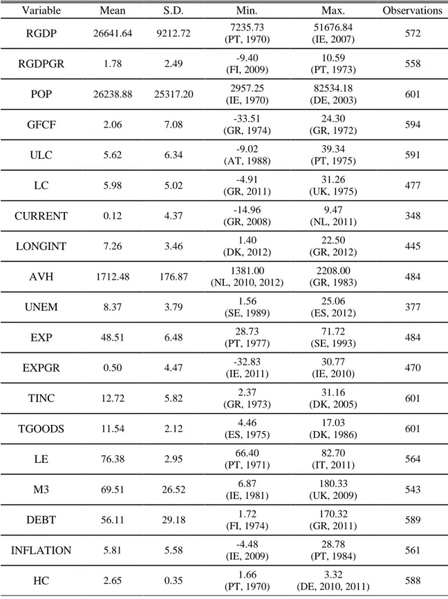
statistics for all variables can be found in Table A1, in Appendix A.11
7 This dataset is available in the following website: http://stats.oecd.org/#
8 Data is available to download in the following website:
http://econ.worldbank.org/WBSITE/EXTERNAL/EXTDEC/EXTRESEARCH/0,,contentMDK:20696167 ~pagePK:64214825~piPK:64214943~theSitePK:469382,00.html
9 The referred is available to download in http://www.rug.nl/research/ggdc/data/penn-world-Table 10 The collected variables are available in
http://www.reinhartandrogoff.com/data/browse-by-topic/topics/7/. I would like to thank to Mr. Kenneth S. Rogoff who, due to lack of data in the referred website, provided me such data.
11 It is important to highlight that some variables which are the logarithmic growth rates (computed by the
author) of those variables not presented in this sub-section, are, in fact, shown in the Table of the descriptive statistics. To identify those variables, the suffix “GR” is added in the final of the respective variable acronym.
18 4. Empirical Analysis
For this analysis, we use two dependent variables: the real per capita GDP annual growth rate and the 5-year average of real per capita GDP growth rates. In the latter case the use of that variable takes into account the cyclical fluctuations in the real GDP path. In this study we use several explanatory variables to understand the behaviour of economic growth in the presence of public debt, as described before in sub-section 3.3. Since government debt will be interacting with different types of variables, we have decided to group them in 4 areas: monetary variables, namely interest rates; public finance variables; institutional variables; and macroeconomic variables. The variables used are presented in each table of results, with the respective code previously reported. For reasons of parsimony, we only show four tables in this section, namely regarding to some results where annual growth rates is the dependent variable. The other results are demonstrated in Appendix B.
4.1. Debt-growth relationship
Looking at all the results we can confirm the existence of the β-convergence process. The expected negative coefficient for the real per capita GDP is obtained and, in most of the cases, that coefficient is statistically significant at 99% level, meaning that the countries used in our sample converge themselves for their own steady-state in the analysed time span. In the case of 5-year average of economic growth there are some coefficients which have a positive signal but once they do not have any statistical significance for growth (at least a 90% level of significance) the relevance of those coefficients is not discussed.
19
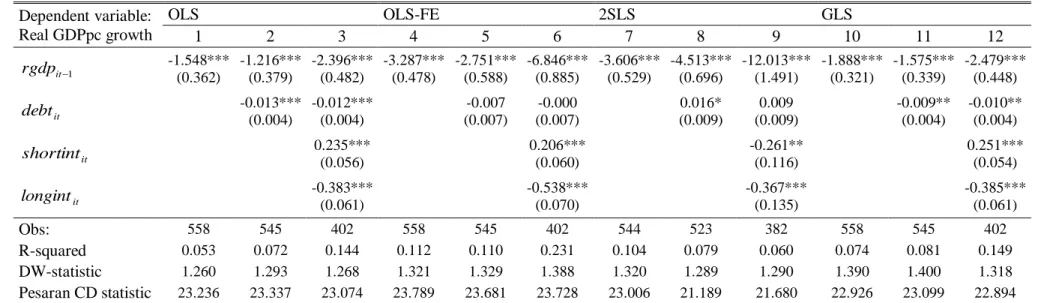
In both cases of annual and 5-year average growth rates we obtain the expected negative sign for the debt coefficient. The detrimental effect of the debt-to-GDP ratio is around -0.01% for each level of 1% of government debt. For example, the level of debt
in Greece in 2011, which was about 170.32%,12 has a negative impact of about -1.7%.
Regarding the interest rates variables, the short-term nominal interest rate presents a statistical significance, in the majority of the regressions, with a positive sign at the 99% level in both cases of annual and 5-year average growth rates. Perhaps, it means that an increase in short-term interests could lead to a higher saving and thus, to a greater capital formation in order to leverage the growth rates in the short term. On the other hand, long-term interest rates have a negative sign. These impacts of both interest
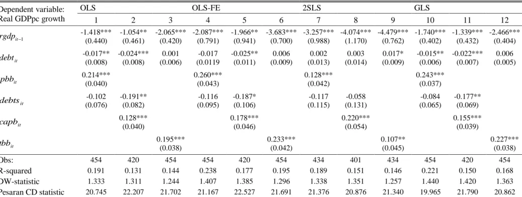
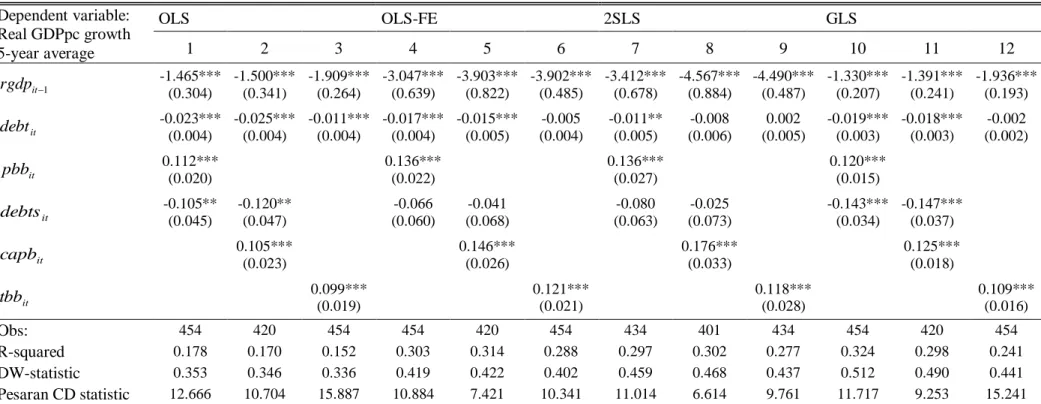
rates can be seen in Table 1.13
Regarding the results of the influence of debt on real growth, interacting with public finance variables, the main factor to highlight is the debt service coefficient. In fact, the results in all regressions exhibit a large detrimental impact for growth when
compared with debt variable by 10 times, in absolute terms (see Table B4).14 The
primary budget balance, the cyclically adjusted primary balance and the total budget balance have the expected positive sign, which follows the idea of a balanced public finances that contribute positively for economic growth.
12 This information was retrieved in Appendix A – Data Statistics.
13 Other results regarding monetary variables are available in Tables B1, B2 and B3 in Appendix B. 14 In Appendix B Tables B4, B5 and B6 also show the results related with public finance variables.
20
Table 1: Growth equations with linear debt effect on real GDP growth rate and with monetary variables.
Dependent variable: Real GDPpc growth OLS OLS-FE 2SLS GLS 1 2 3 4 5 6 7 8 9 10 11 12 1 it rgdp -1.548*** (0.362) -1.216*** (0.379) -2.396*** (0.482) -3.287*** (0.478) -2.751*** (0.588) -6.846*** (0.885) -3.606*** (0.529) -4.513*** (0.696) -12.013*** (1.491) -1.888*** (0.321) -1.575*** (0.339) -2.479*** (0.448) it debt -0.013*** (0.004) -0.012*** (0.004) -0.007 (0.007) -0.000 (0.007) 0.016* (0.009) 0.009 (0.009) -0.009** (0.004) -0.010** (0.004) it shortint 0.235*** (0.056) 0.206*** (0.060) -0.261** (0.116) 0.251*** (0.054) it longint -0.383*** (0.061) -0.538*** (0.070) -0.367*** (0.135) -0.385*** (0.061) Obs: 558 545 402 558 545 402 544 523 382 558 545 402 R-squared 0.053 0.072 0.144 0.112 0.110 0.231 0.104 0.079 0.060 0.074 0.081 0.149 DW-statistic 1.260 1.293 1.268 1.321 1.329 1.388 1.320 1.289 1.290 1.390 1.400 1.318 Pesaran CD statistic 23.236 23.337 23.074 23.789 23.681 23.728 23.006 21.189 21.680 22.926 23.099 22.894 Notes: *, ** and *** represent statistical significance at 10, 5 and 1 percent level respectively. The robust standard errors are in parentheses. The White diagonal covariance matrix is used in order to assume residual heteroskedasticity, except for the Generalized Least Squares methodology. DW-statistic is the Durbin-Watson statistic and Pesaran CD statistic is the Pesaran cross-section dependence statistic.
21
On the other hand, institutional variables demonstrate an evidence in which countries belonging to Eurozone suffer a growth decrease of more than -0.5%, existing even cases where this event presents an even more negative impact of -1%. The number of crises happened in a certain year has a negative sign, as we could expect.
In addition, banking crisis has the most negative crisis effect for economic growth, representing a downward dynamics on growth of more than -1%. Although stock market crashes are bad events for growth, they present themselves not statistically significant. Inflation crises and currency crises have also an undesirable and expected effect, having the latter crises about a half of the negative effect that inflation crises have.
Another important result to mention is the positive impact of the Stability and Growth Pact, which rely on a conclusion that the signature of this agreement lead to a better behave of public finances and, consequently, to a positive impact on economic growth.
However, the Maastricht Treaty has a dubious effect on the dependent variable, and in most cases, it not significant at a minimum of 90%, turning into a variable which does not need our moderation.
22
Table 2: Growth equations with debt linear effect on real GDP growth rate and with institutional variables.
Dependent variable: Real GDPpc growth OLS OLS-FE 2SLS GLS 1 2 3 4 5 6 7 8 9 10 11 12 1 it rgdp -1.486*** (0.373) -1.328*** (0.375) -1.466*** (0.430) -2.872*** (0.600) -2.909*** (0.587) -5.784*** (0.958) -4.575*** (0.722) -4.291*** (0.696) -8.042*** (1.133) -1.629*** (0.337) -1.415*** (0.312) -1.644*** (0.370) it debt -0.007** (0.004) -0.004 (0.004) -0.004 (0.004) -0.000 (0.007) 0.009 (0.007) 0.010 (0.008) 0.024*** (0.008) 0.031*** (0.008) 0.031*** (0.008) -0.006* (0.003) -0.003 (0.003) -0.002 (0.003) it y crisestall -0.971*** (0.140) -0.928*** (0.147) -0.873*** (0.156) -0.794*** (0.124) it inflationc -1.480* (0.785) -1.501* (0.789) -1.444* (0.771) -1.371* (0.744) -1.383* (0.820) -1.355* (0.793) -0.841 (0.762) -0.896 (0.770) it tc stockmarke -0.236 (0.217) -0.199 (0.218) -0.116 (0.223) -0.077 (0.221) 0.115 (0.238) 0.106 (0.238) 0.010 (0.194) 0.044 (0.197) it currencyc -0.752** (0.323) -0.784** (0.331) -0.676** (0.335) -0.721** (0.316) -0.595* (0.352) -0.696** (0.333) -0.705** (0.296) -0.731** (0.307) it bankingc -2.149*** (0.312) -2.070*** (0.315) -2.225*** (0.315) -1.977*** (0.316) -2.451*** (0.325) -2.122*** (0.327) -2.048*** (0.295) -1.975*** (0.297) it euro -0.836*** (0.312) -0.605* (0.331) -0.525 (0.347) -0.792*** (0.286) it sgp 0.726** (0.362) 1.429*** (0.356) 1.898*** (0.367) 0.775** (0.345) it maas -0.032 (0.308) 0.670* (0.349) 0.618* (0.367) -0.064 (0.295) Obs: 517 515 515 517 515 515 495 493 493 517 515 515 R-squared 0.134 0.176 0.185 0.155 0.201 0.233 0.126 0.183 0.217 0.122 0.181 0.192 DW-statistic 1.607 1.597 1.608 1.621 1.614 1.628 1.569 1.576 1.580 1.634 1.637 1.648 Pesaran CD statistic 20.648 3.983 4.495 21.235 7.314 8.103 18.856 9.015 9.348 20.886 5.621 6.187 Notes: *, ** and *** represent statistical significance at 10, 5 and 1 percent level respectively. The robust standard errors are in parentheses. The White diagonal covariance matrix is used in order to assume residual heteroskedasticity, except for the Generalized Least Squares methodology. DW-statistic is the Durbin-Watson statistic and Pesaran CD statistic is the Pesaran cross-section dependence statistic.
23
Analysing the results of the macroeconomic variables, presented in Table 4,15 we
can observe that taxation on capital and profits present a negative sign when statistically significant. Thus, it allows us to speculate about the possible burden of this type of taxation, given that there would remain fewer wealth to generate more capital. On the other side, the values obtained for taxation on goods and services do not follow the same constant pattern because they assume positive and negative statistical results. For that reason, it is no object of discussion in this analysis.
Another interesting result relies on the growth rate of credit to private sector. This variable induces a decline of economic growth by more than 0.01% per each amount of 1% increase of credit. According to Sassi & Gasmi (2014), this result is due to the larger proportion of credit conceived to households relatively to firms. The values of this paper confirms our results, in the sense that the households’ credit effect on real
per capita GDP is negative and it has a major role, in absolute terms, on economic
growth. Contrarely to firms in which credit is used for productive investment, the growth of credit to households is followed by financial instability as well as the increase of external debt. A positive effect for the growth rate of per capita GDP is given by several variables, namely, annual growth rate of gross fixed capital formation, current account balance, trade openness, average hours worked and urbanization rate. Contrarily to these results, whenever liquid liabilities, life expectancy, the level of government expenditures and its annual growth rate, and unemployment rate are significant in statistical terms, they have an undesirable effect on economic growth.
According to economic theory, the output gap and total factor productivity variables present positive coefficients when the same are significant. In fact, a 1%
24
output gap beyond potential GDP will contribute for more than 0.5% of per capita GDP growth rate. Inflation, which is considered as a detrimental factor for real economic growth rate, follows a consistent pattern in the majority of cases, presenting the expected negative effect on growth in the regressions displayed by Tables 4, B10, B11 and B12.
Other results that must be highlighted are the fact that the level of population and the labour compensation per unit of labour have an important and positive explanation in the long-run (these results are just valid for regressions with 5-year average per capita growth rate as dependent variable). Even though the unit labour costs variable is significant, both in the short and long term, its effect differs across time: in annual terms, labour costs present as being negative for growth, but in a 5-year average, they achieve a positive result for economic path. Lastly, the human capital and the stock of capital do not present a constant sign across the several econometric tests, which do not lead us to a feasible conclusion for these two variables.
4.2. Non-linarities of government debt on growth
As proved in the previous section, government debt has a negative effect on growth, both in the short and long terms. Despite that behaviour, there are some articles which study the existence of a non-linear relationship between the debt ratio and the economic performance. As already mentioned, the evidence of an inverted U-shape is also detailed in this thesis. The threshold is associated with the level of government debt that most contributes to the economic growth. Supposing that we have a threshold of 60% of public debt-to-GDP ratio, for each additional value of 1% on debt from that point forward, the positive effect of debt on growth will consequently be lower, as its
25
levels continue to increase. These positive threshold effects may be related to the preference of government in releasing capital for the private sector and not relying only on taxation. Through this way, governments are able to stimulate investment and consumption by companies and households.
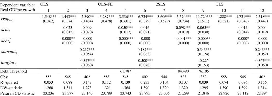
By adding the squared debt-to-GDP variable, equation (2) allows us not only to study the non-linearity effect of government debt on economic growth but also to analyse the values for the government debt thresholds. First, we decide to calculate these thresholds only when both coefficients of debt and debt squared are statistically significant, at least of 90% level; second, we derive equation (2), as demonstrated below in equation (3); third, we equalize to zero that first-derivative and get equation (4):
(3) ) , ( ) ( ) , ( 2 2 3 2 1 1 0 2 it it it i t it it j it it it it it it it D D D D x y D D g (4) 3 2 3 2 2 2 0 Dit Dit .
To obtain the debt thresholds, we expect a negative3, i.e., a concave function
of public debt effect on economic growth – the inverted U-shape. In Tables 3 and 4 we
present some results for thresholds.16
Although we obtain threshold values that go from 49.49% to 108.24%, which depend on the econometric method used and on the set of variables, on average, the most observed threshold value is about 74.84% for annual growth rates.
For the 5-year average growth rate, we obtain a maximum effect of debt on growth of 74.44%, a similar value to the one we got on annual growth rates.
16 Appendix B also exhibits the other obtained results for debt on the tables containing the debt-squared
26
Table 3: The non-linearity effect of public debt on real GDP growth rate, with public finance variables.
Dependent variable: Real GDPpc growth OLS OLS-FE 2SLS GLS 1 2 3 4 5 6 7 8 9 10 11 12 1 it rgdp -1.912*** (0.441) -1.562*** (0.441) -2.531*** (0.438) -4.134*** (0.827) -4.320*** (0.884) -5.187*** (0.744) -5.479*** (1.037) -7.260*** (1.174) -5.791*** (0.794) -2.260*** (0.401) -1.789*** (0.425) -2.998*** (0.409) it debt 0.061*** (0.016) 0.051*** (0.017) 0.081*** (0.017) 0.095*** (0.020) 0.092*** (0.021) 0.121*** (0.018) 0.128*** (0.026) 0.169*** (0.030) 0.135*** (0.022) 0.057*** (0.014) 0.046*** (0.016) 0.081*** (0.016) 2 it debt -0.001*** (0.000) -0.000*** (0.000) -0.001*** (0.000) -0.001*** (0.000) -0.001*** (0.000) -0.001*** (0.000) -0.001*** (0.000) -0.001*** (0.000) -0.001*** (0.000) -0.000*** (0.000) -0.000*** (0.000) -0.001*** (0.000) it pbb 0.258*** (0.045) 0.309*** (0.045) 0.193*** (0.043) 0.290*** (0.038) it debts -0.030 (0.066) -0.121* (0.069) 0.104 (0.086) 0.054 (0.088) 0.139 (0.103) 0.293*** (0.112 -0.045 (0.062) -0.144** (0.065) it capb 0.186*** (0.042) 0.254*** (0.046) 0.331*** (0.054) 0.208*** (0.041) it tbb 0.244*** (0.042) 0.303*** (0.044) 0.191*** (0.044) 0.274*** (0.038) Debt Threshold 59.647 51.813 75.585 70.533 66.259 78.990 82.339 83.684 84.117 58.299 49.493 77.063 Obs: 454 420 454 454 420 454 434 401 434 454 420 454 R-squared 0.250 0.185 0.211 0.308 0.247 0.296 0.269 0.216 0.264 0.274 0.195 0.228 DW-statistic 1.420 1.405 1.333 1.501 1.505 1.455 1.428 1.471 1.414 1.461 1.451 1.365 Pesaran CD statistic 20.583 22.070 21.259 20.951 22.621 20.886 20.885 19.977 20.798 19.632 21.547 20.265 Notes: *, ** and *** represent statistical significance at 10, 5 and 1 percent level respectively. The robust standard errors are in parentheses. The White diagonal covariance matrix is used in order to assume residual heteroskedasticity, except for the Generalized Least Squares methodology. DW-statistic is the Durbin-Watson statistic and Pesaran CD statistic is the Pesaran cross-section dependence statistic.
27
Analysing, on average, the results of each group of variables for annual growth rates, we get a maximum threshold for institutional variables of 95.84%, unlike for the macroeconomic variables case, which only obtain a lower value rounding 66.21%. The average thresholds obtained for the remaining variables, monetary and public finance, are 74.16% and 69.82%, respectively.
In the case of 5-year average growth rates, we reach to a high threshold of 91.27% for institutional variables (not on average, once there is only one result for this sample). In the case of public finance variables we get the minimum mean threshold, rounding the 63.11%.
28 Dependent variable: Real GDPpc growth OLS OLS-FE 2SLS GLS 1 2 3 4 5 6 7 8 9 10 11 12 1 it rgdp -1,975*** (0,714) -0,859*** (0,260) -2,381*** (0,788) -35,706*** (3,558) -1,477 (0,938) -8,682*** (1,982) -19,918*** (4,317) 1,906 (22,886) -7,140*** (2,005) -1,959*** (0,646) -0,817*** (0,245) -2,338*** (0,657) it debt 0,042** (0,018) -0,003 (0,009) 0,005 (0,022) -0,012 (0,023) -0,009 (0,010) 0,047* (0,025) 0,105*** (0,027) -0,040 (0,168) 0,048** (0,024) 0,044** (0,018) -0,005 (0,008) 0,001 (0,019) 2 it debt -0,000*** (0,000) (0,000) -0,000 -0,000** (0,000) (0,000) -0,000 (0,000) -0,000 -0,000*** (0,000) -0,001*** (0,000) (0,001) 0,000 -0,000*** (0,000) -0,000*** (0,000) (0,000) -0,000 -0,000** (0,000) it pbb 0,259*** (0,047) -0,111 (0,076) 0,280*** (0,040) -0,110 (0,076) 0,220*** (0,047) -0,107 (0,077) 0,273*** (0,042) -0,117*** (0,045) it debts -0,038 (0,072) -0,344*** (0,095 0,186*** (0,071) -0,179 (0,135) 0,385*** (0,093) -0,200 (0,136) -0,042 (0,071) -0,337*** (0,078) it tinc 0,014 (0,029) -0,105* (0,057) -0,215*** (0,071) -0,005 (0,026) it tgoods -0,135* (0,081) 0,150 (0,110) 0,533*** (0,189) -0,049 (0,076) ) log(kit1 -0,260** (0,130) 11,709*** (1,914) 3,468 (2,263) -0,265** (0,125) ) log(tfpit 4,176*** (1,267) 39,517*** (3,113) 21,621*** (4,156) 4,278*** (1,269) ) log(hcit 0,632 (1,635) 25,501 (2,409) 12,357*** (3,237) -0,201 (1,506) it inflation 0,103*** (0,036) -0,309*** 0,114 0,085** (0,034) -0,268** (0,124) -0,223 (0,354) -0,265** (0,122) 0,112*** (0,030) -0,348*** (0,081) ) log(popit 0,020 (0,065) -0,472 (2,616) 2,010 (18,134) 0,005 (0,059) it credit -0,015** (0,007) -0,017** (0,008) -0,1585 (0,610) -0,011* (0,006) it m3 -0,003 (0,003) -0,000 (0,004) 0,004 (0,050) -0,001 (0,002)
29 Real GDPpc growth 1 2 3 4 5 6 7 8 9 10 11 12 it le -0,165*** (0,041) -0,130 (0,090) -0,365 (0,979) -0,173*** (0,036) it gfcf 0,258*** (0,012) 0,255*** (0,012) 0,333 (0,217) 0,261*** (0,010) it ulc -0,192*** (0,033) -0,211*** (0,033) 0,063 (0,445) -0,188*** (0,027) it current 0,122*** (0,041) 0,130** (0,052) 0,128** (0,053) 0,105** (0,032) it tradeope 0,010** (0,005) 0,014 (0,014) 0,009 (0,015) 0,005 (0,004) it exp -0,034* (0,019) -0,083 (0,064) -0,076 (0,064) -0,033** (0,016) it expgr -0,210*** (0,064) -0,164** (0,066) -0,169** (0,067) -0,302*** (0,038) it unem -0,007 (0,043) -0,098 (0,078) -0,078 (0,078) -0,035 (0,039) it outputgap 0,551*** (0,085) 0,593*** (0,088) 0,596*** (0,089) 0,490*** (0,056) it avh 0,004*** (0,001) 0,005 (0,004) 0,006 (0,004) 0,004*** (0,001) it urb 0,031** (0,013) 0,134*** (0,053) 0,120** (0,053) 0,040*** (0,012) it lc 0,009 (0,060) -0,079 (0,068) -0,071 (0,067) 0,032 (0,053) Debt Threshold 53.242 59.714 102.472 60.169 55.460 Obs: 440 479 273 440 479 273 420 453 272 440 479 273 R-squared 0,248 0,735 0,658 0,558 0,753 0,710 0,469 0,430 0,709 0,265 0,747 0,724 DW-statistic 1,440 1,738 1,654 1,107 1,790 1,627 1,400 2,081 1,675 1,469 1,702 1,693 Pesaran CD statistic 20,045 7,307 13,983 13,669 7,199 14,980 17,429 4,473 15,209 19,483 7,742 10,146 Notes: *, ** and *** represent statistical significance at 10, 5 and 1 percent level respectively. The robust standard errors are in parentheses. The White diagonal covariance matrix is used in order to assume residual heteroskedasticity, except for the Generalized Least Squares methodology. DW-statistic is the Durbin-Watson statistic and Pesaran CD statistic is the Pesaran cross-section dependence statistic.
30 5. Conclusions
Today the academia and both sides of political spectrums discuss the role of government debt on economic growth, and it seems that we live in a “time of debt”. But this “time of debt” we live in arose, mainly, when a certain kind of crisis recently emerged in 2007 with the bankruptcy of the biggest financial companies in the world, making us experience all of its consequences. What appeared to be a banking and financial crisis, it has become a sovereign debt crisis, affecting in particular the peripheral Eurozone countries.
In this thesis we have analysed the effect government debt has on real per capita GDP growth, annually and in 5-year average rates. We have also determined the effect of other variables while interacting with the sovereign debt-to-GDP ratio.
For 14 European countries and 43 years (1970-2012) we can conclude that, as usually affirmed, debt is negative for growth, both in short and long-terms. In addition to this fact, we highlight the process of convergence between our countries’ sample. Looking at interest rates, short-term interest rate has a positive effect on growth, contrarily to the case of long-term rate. When we analyse both debt-to-GDP ratio and debt service variables, the last one has a much more negative effect on economic performance when compared with debt.
Contrarily to the Stability and Growth Pact signature, for which we have found evidence of positive contributions to economy once it had a disciplinable effect on public finances, the signature of the Maastricht treaty as well as the introduction of euro in some countries were some institutional events that led to a lower economic growth behaviour. Also, we stress the fact of banking crisis be the worst type of crisis that can occur in an economy.
31
Another important conclusion is that when debt interacts with macroeconomic variables we find evidences of unfavourable effects of taxation on capital and profits, the growth of credit to private sector as well as government expenditures. On the other hand, total factor productivity, current account balance and urbanization are some variables which contribute positively to growth.
Finally, we provide results showing the existence of an inverted U-shape relationship between debt ratio and economic growth. During the computation of the two average thresholds for this non-linear relationship, we have reached for annual and 5-year average growth rate thresholds of 75% and 74%, respectively. Therefore, and according to these values, government could keep debt levels under those values in order to avoid sovereign debt crises, like the one most countries in our sample are experiencing recently.
Although the undesirable debt effect, governments have the trade-off the increment of debt to stimulate aggregate demand and, posteriorly, growth. Debt should not be the main point in political and academic agenda if each economy had the sufficient and structural mechanisms to deal with it. Concentrating on how efficiently each economy could improve its economic path, surely is the best way to prevent the negative speculations about sovereign debt by financial markets, as we can see from the case of Greece, Ireland and Portugal – countries that have experienced a severe time of economic austerity.
32 References
Afonso, A., 2005. Ricardian fiscal regimes in the European Union. Empirica, 35(3), pp. 313-334.
Afonso, A. & Jalles, J. J., 2013. Growth and productivity: The role of government debt.
International Review of Economics & Finance, Volume 25, p. 384–407.
Afonso, A. & Jalles, J. T., 2012. Fiscal volatility, financial crises and growth. Applied
Economics Letters, 19(18), pp. 1821-1826.
Barro, R. J. & Sala-i-Martin, X., 2004. Economic Growth. 2nd ed. s.l.:MIT Press.
Baum, A., Checherita-Westsphal, C. & Rohter, P., 2013. Debt and growth: New evidence for the euro area. Journal of International Money and Finance, 32(0), pp. 809 - 821.
Beck, T., Demirgüç-Kunt, A. & Levine, R., 2009. Financial Institutions and Markets Across Countries and over Time: Data and Analysis. World Bank Policy Research
Working Paper 4943.
Breusch, T. & Pagan, A. R., 1980. The Lagrange Multiplier test and its applications to model specification in econometrics. Econometrics Issue, 47(1), pp. 239-253.
Buchanan, J. M., 1966. The icons of public debt. The Journal of Finance, 21(3), pp. 544-546.
Campos, C. F., Jaimovich, D. & Panizza, U., 2006. The unexplained part of public debt.
33
Cecchetti, S. G., Mohanty, M. S. & Zampolli, F., 2011. The real effects of debt. BIS
Working Papers, Issue 352, pp. 1-33.
Checherita-Westphal, C. & Rother, P., 2012. The impact of high government debt on economic growth and its channels: An empirical investigation for the euro area.
European Economic Review, 56(7), pp. 1392 - 1405.
Chudik, A., Pesaran, H. & Tosetti, E., 2009. Weak and strong cross section dependence and estimation of large panels. ECB Working Series, Issue 1100.
Diamond, P. A., 1965. National Debt in a Neoclassical Growth Model. American
Economic Review, 55(5), pp. 1126-1150.
Elgin, C. & Uras, B. R., 2012. Public debt, sovereign default risk and shadow economy.
Journal of Financial Stability, Issue 0, pp. 1572-3089.
Feenstra, R. C., Inklaar, R. & Timmer, M. P., 2013. The Next Generation of the Penn World Table.
Feldstein, M., 1985. Debt and taxes in the theory of public finance. Journal of Public
Economics, 28(2), pp. 233-245.
Fincke, B. & Greiner, A., 2011. Debt Sustainability in Selected Euro Area Countries: Empirical Evidence Estimating Time-Varying Parameters. Studies in Nonlinear
Dynamics & Econometrics, 15(3), pp. 1-21.
Fölster, S. & Henrekson, M., 2001. Growth effects of government expenditure and taxation in rich countries. European Economic Review, 45(8), pp. 1501-1520.
Gnegne, Y. & Jawadi, F., 2013. Boundedness and nonlinearities in public debt dynamics: A TAR assessment. Economic Modelling, 34(0), pp. 154-160.
34
Greiner, A., 2012. Public debt in a basic endogenous growth model. Economic
Modelling, 29(4), pp. 1344 - 1348.
Greiner, A., 2013. Sustainable Public Debt and Economic Growth under Wage Rigidity.
Metroeconomics, 64(2), p. 272–292.
Gruber, J. W. & Kamin, S. B., 2012. Fiscal Positions and Government Bond Yields in OECD Countries. Journal of Money, Credit and Banking, Volume 44, p. 1563–1587.
Heylen, F., Hoebeeck, A. & Buyse, T., 2013. Government efficiency, institutions, and the effects of fiscal consolidation on public debt. European Journal of Political
Economy, 31(0), pp. 40-59.
Kolluri, B. & Wahab, M., 2007. Asymmetries in the conditional relation of government expenditure and economic growth. Applied Economics, 39(18), pp. 2303-2322.
Kourtellos, A., Stengos, T. & Tan, C. M., 2013. The effect of public debt on growth in multiple regimes. Journal of Macroeconomics, pp. 1-9.
Kumar, M. S. & Jaejoon, W., 2010. Public Debt and Growth. IMF Working Paper, Volume WP/10/174.
Leão, P., 2013. The Effect of Government Spending on the Debt-to-GDP Ratio: Some Keynesian Arithmetic. Metroeconomica, 64(3), pp. 448-465.
Martin, F. M., 2009. A positive theory of government debt. Review of Economic
Dynamics, 12(4), p. 608–631.
Pesaran, M., 2006. Estimation and Inference in Large Heterogeneous Panels with a Multifactor Error Structure. Econometrica, 74(4), pp. 967-1012.
35
Reinhart, C. M. & Rogoff, K. S., 2009. This Time Is Different: Eight Centuries of
Financial Folly. Princeton, NJ: Princeton University Press.
Reinhart, C. M. & Rogoff, K. S., 2010. Growth in a Time of Debt. American Economic
Review, 100(2), pp. 573 - 578.
Reinhart, C. M. & Rogoff, K. S., 2011. The Forgotten History of Domestic Debt. The
Economic Journal, 121(552), pp. 319-350.
Sarafidis, V. & Wansbeek, T., 2010. Cross-sectional Dependence in Panel Data Analysis. MPRA Paper.
Sassi, S. & Gasmi, A., 2014. The effect of enterprise and household credit on economic growth: New evidence from European union countries. Journal of Macroeconomics, Issue 39, pp. 226-231.
Schclarek, A., 2004. Debt and Economic Growth in Developing and Industrial Countries. Lund University, Department of Economics Working Papers, Dec.
Teica, R. A., 2012. Analysis of the Public Debt Sustainability in the Economic and Monetary Union. Procedia Economics and Finance, 3(0), pp. 1081-1087.
Wahab, M., 2004. Economic growth and government expenditure: evidence from a new test specification. Applied Economics, 36(19), pp. 2125-2135.
Westerlund, J. & Prohl, S., 2010. Panel cointegration tests of the sustainability hypothesis in rich OECD countries. Applied Economics, 42(11), pp. 1355-1364.
Wigger, B. U., 2009. A note on public debt, tax-exempt bonds, and Ponzi games.
36
Wooldridge, J. M., 2009. Introductory Econometrics: A Modern Approach. 4th ed. Canada: South-Western CENGAGE Learning.
Wright, D. M., 1943. Moulton's The New Philosophy of Public Debt. American
37 Appendix A – Data Statistics
Table A1: Summary statistics for the panel 1970-2012.
Variable Mean S.D. Min. Max. Observations
RGDP 26641.64 9212.72 7235.73 (PT, 1970) 51676.84 (IE, 2007) 572 RGDPGR 1.78 2.49 -9.40 (FI, 2009) 10.59 (PT, 1973) 558 POP 26238.88 25317.20 2957.25 (IE, 1970) 82534.18 (DE, 2003) 601 GFCF 2.06 7.08 -33.51 (GR, 1974) 24.30 (GR, 1972) 594 ULC 5.62 6.34 -9.02 (AT, 1988) 39.34 (PT, 1975) 591 LC 5.98 5.02 -4.91 (GR, 2011) 31.26 (UK, 1975) 477 CURRENT 0.12 4.37 -14.96 (GR, 2008) 9.47 (NL, 2011) 348 LONGINT 7.26 3.46 1.40 (DK, 2012) 22.50 (GR, 2012) 445 AVH 1712.48 176.87 1381.00 (NL, 2010, 2012) 2208.00 (GR, 1983) 484 UNEM 8.37 3.79 1.56 (SE, 1989) 25.06 (ES, 2012) 377 EXP 48.51 6.48 28.73 (PT, 1977) 71.72 (SE, 1993) 484 EXPGR 0.50 4.47 -32.83 (IE, 2011) 30.77 (IE, 2010) 470 TINC 12.72 5.82 2.37 (GR, 1973) 31.16 (DK, 2005) 601 TGOODS 11.54 2.12 4.46 (ES, 1975) 17.03 (DK, 1986) 601 LE 76.38 2.95 66.40 (PT, 1971) 82.70 (IT, 2011) 564 M3 69.51 26.52 6.87 (IE, 1981) 180.33 (UK, 2009) 543 DEBT 56.11 29.18 1.72 (FI, 1974) 170.32 (GR, 2011) 589 INFLATION 5.81 5.58 -4.48 (IE, 2009) 28.78 (PT, 1984) 561 HC 2.65 0.35 1.66 (PT, 1970) 3.32 (DE, 2010, 2011) 588
38
Variable Mean S.D. Min. Max. Observations
K 1866761.22 2099888.36 41184.71 (IE, 1970) 8873920.00 (DE, 2011) 588 TFP 0.94 0.11 0.63 (FI, 1971) 1.19 (ES, 1989) 588 URB 72.29 12.32 38.80 (PT, 1970) 97.51 (BE, 2012) 602 CREDIT 83.31 43.42 17.99 (GR, 1970) 232.10 (IE, 2009) 598 SHORTINT 7.52 4.99 0.57 (EMU, 2012) 24.56 (GR, 1994) 572 CAPB 0.96 3.35 -25.03 (IE, 2012) 10.46 (DK, 1986) 447 OUTPUTGAP 0.09 2.35 -11.92 (GR, 2012) 7.71 (PT, 1972) 580 PBB 0.84 3.59 -27.46 (IE, 2010) 11.62 (DK, 1986) 484 TBB -3.27 4.22 -30.61 (IE, 2010) 7.73 (FI, 1976) 484 DEBTS 4.11 2.51 -12.60 (IT, 1993) 12.60 (FI, 1975) 484 TRADEOPE 72.19 33.21 25.79 (ES, 1970) 191.37 (IE, 2012) 602
39
Table B1: The non-linearity effect of public debt on real GDP growth rate, with monetary variables.
Dependent variable: Real GDPpc growth OLS OLS-FE 2SLS GLS 1 2 3 4 5 6 7 8 9 10 11 12 1 it rgdp -1.548*** (0.362) -1.443*** (0.374) -2.390** (0.484) -3.287*** (0.478) -3.536*** (0.601) -6.734*** (0.879) -3.606*** (0.529) -5.570*** (0.734) -11.720*** (1.511) -1.888*** (0.321) -1.731*** (0.346) -2.518*** (0.447) it debt 0.023 (0.015) 0.009 (0.020) 0.050*** (0.017) 0.016 (0.021) 0.098*** (0.019) 0.065** (0.030) 0.014 (0.014) 0.004 (0.019) 2 it debt -0.000** (0.000) (0.000) -0.000 -0.000*** (0.000) (0.000) -0.000 -0.001*** (0.000) -0.000** (0.000) -0.000* (0.000) (0.000) -0.000 it shortint 0.217*** (0.054) 0.187*** (0.063) -0.343*** (0.124) 0.243*** (0.052) it longint -0.347*** (0.060) -0.500*** (0.078) -0.225 (0.153) -0.367*** (0.060) Debt Threshold 61.787 84.490 76.195 Obs: 558 545 402 558 545 402 544 523 382 558 545 402 R-squared 0.053 0.088 0.147 0.112 0.139 0.233 0.104 0.107 0.039 0.074 0.086 0.156 DW-statistic 1.260 1.311 1.273 1.321 1.364 1.390 1.320 1.320 1.295 1.390 1.399 1.314 Pesaran CD statistic 23.236 23.377 23.140 23.789 23.743 23.795 23.006 21.299 21.846 22.926 23.112 22.894 Notes: *, ** and *** represent statistical significance at 10, 5 and 1 percent level respectively. The robust standard errors are in parentheses. The White diagonal covariance matrix is used in order to assume residual heteroskedasticity, except for the Generalized Least Squares methodology. DW-statistic is the Durbin-Watson statistic and Pesaran CD statistic is the Pesaran cross-section dependence statistic.
40
Table B2: Growth equations with linear debt effect in real GDP growth rate and with monetary variables, 5-year average.
Dependent variable: Real GDPpc growth 5-year average OLS OLS-FE 2SLS GLS 1 2 3 4 5 6 7 8 9 10 11 12 1 it rgdp -1.548*** (0.183) -1.208*** (0.189) -1.397*** (0.315) -3.450*** (0.314) -2.787*** (0.334) -4.075*** (0.511) -3.832*** (0.346) -3.820*** (0.363) -5.846*** (0.706) -1.706*** (0.144) -1.419*** (0.156) -1.798*** (0.262) it debt -0.017*** (0.003) -0.011*** (0.003) -0.011*** (0.003) -0.004 (0.004) -0.000 (0.004) 0.008** (0.004) -0.009*** (0.002) -0.009*** (0.002) it shortint 0.121*** (0.027) 0.090*** (0.029) 0.071 (0.051) 0.076** (0.031) it longint -0.147*** (0.035) -0.229*** (0.037) -0.282*** (0.058) -0.111*** (0.041) Obs: 558 545 402 558 545 402 544 523 382 558 545 402 R-squared 0.082 0.136 0.182 0.245 0.254 0.301 0.244 0.247 0.286 0.180 0.203 0.223 DW-statistic 0.385 0.415 0.462 0.468 0.480 0.517 0.473 0.480 0.508 0.404 0.417 0.443 Pesaran CD statistic 15.825 16.638 14.553 7.455 10.715 10.679 7.221 7.384 6.549 15.088 15.277 13.922 Notes: *, ** and *** represent statistical significance at 10, 5 and 1 percent level respectively. The robust standard errors are in parentheses. The White diagonal covariance matrix is used in order to assume residual heteroskedasticity, except for the Generalized Least Squares methodology. DW-statistic is the Durbin-Watson statistic and Pesaran CD statistic is the Pesaran cross-section dependence statistic.
41
Table B3: The non-linearity effect of public debt on real GDP growth rate, with monetary variables, 5-year average.
Dependent variable: Real GDPpc growth 5-year average OLS OLS-FE 2SLS GLS 1 2 3 4 5 6 7 8 9 10 11 12 1 it rgdp -1.548*** (0.183) -1.250*** (0.197) -1.393*** (0.315) -3.450*** (0.314) -3.016*** (0.345) -4.023*** (0.498) -3.832*** (0.346) -4.120*** (0.375) -5.831*** (0.707) -1.706*** (0.144) -1.495*** (0.162) -1.789*** (0.264) it debt -0.010 (0.008) 0.001 (0.011) 0.006 (0.009) 0.003 (0.011) 0.023** (0.011) 0.011 (0.014) 0.001 (0.006) -0.005 (0.009) 2 it debt -0.000 (0.000) -0.000 (0.000) -0.000** (0.000) -0.000 (0.000) -0.000** (0.000) -0.000 (0.000) -0.000 (0.000) -0.000 (0.000) it shortint 0.110*** (0.030) 0.081*** (0.031) 0.067 (0.058) 0.074** (0.031) it longint -0.125*** (0.041) -0.211*** (0.042) -0.275*** (0.073) -0.104** (0.042) Debt Threshold 68.951 Obs: 558 545 402 558 545 402 544 523 382 558 545 402 R-squared 0.082 0.137 0.184 0.245 0.258 0.302 0.244 0.250 0.286 0.180 0.206 0.220 DW-statistic 0.385 0.416 0.461 0.468 0.483 0.515 0.473 0.483 0.507 0.404 0.419 0.441 Pesaran CD statistic 15.825 16.901 14.811 7.455 9.587 10.315 7.221 6.853 6.421 15.088 15.494 14.045 Notes: *, ** and *** represent statistical significance at 10, 5 and 1 percent level respectively. The robust standard errors are in parentheses. The White diagonal covariance matrix is used in order to assume residual heteroskedasticity, except for the Generalized Least Squares methodology. DW-statistic is the Durbin-Watson statistic and Pesaran CD statistic is the Pesaran cross-section dependence statistic.