The Atmospheric Chemistry and Canopy Exchange Simulation System (ACCESS): model description and application to a temperate deciduous forest canopy

(1)

ACPD

12, 24765–24820, 2012

The Atmospheric Chemistry and Canopy Exchange Simulation System

R. D. Saylor

Title Page

Abstract Introduction

Conclusions References

Tables Figures

◭ ◮

Back Close

Full Screen / Esc

Printer-friendly Version Interactive Discussion

Discussion

P

a

per

|

Dis

cussion

P

a

per

|

Discussion

P

a

per

|

Discussio

n

P

a

per

|

Atmos. Chem. Phys. Discuss., 12, 24765–24820, 2012 www.atmos-chem-phys-discuss.net/12/24765/2012/ doi:10.5194/acpd-12-24765-2012

Atmospheric Chemistry and Physics Discussions

This discussion paper is/has been under review for the journal Atmospheric Chemistry and Physics (ACP). Please refer to the corresponding final paper in ACP if available.

The Atmospheric Chemistry and Canopy

Exchange Simulation System (ACCESS):

model description and application to a

temperate deciduous forest canopy

R. D. Saylor

National Oceanic and Atmospheric Administration, Air Resources Laboratory, Atmospheric Turbulence and Diffusion Division, 456 S. Illinois Ave., Oak Ridge, TN 37830, USA

Received: 15 August 2012 – Accepted: 6 September 2012 – Published: 21 September 2012

Correspondence to: R. D. Saylor ([email protected])

Published by Copernicus Publications on behalf of the European Geosciences Union.

(2)

ACPD

12, 24765–24820, 2012

R. D. Saylor

Title Page

Tables Figures

◭ ◮

Back Close

Full Screen / Esc

Discussion

P

a

per

|

Dis

cussion

P

a

per

|

Discussion

P

a

per

|

Discussio

n

P

a

per

|

Abstract

Forest canopies are primary emission sources of biogenic volatile organic compounds (BVOCs) and have the potential to significantly influence the formation and distribution of secondary organic aerosol (SOA) mass. Biogenically-derived SOA formed as a re-sult of emissions from the widespread forests across the globe may affect air quality 5

in populated areas, degrade atmospheric visibility, and affect climate through direct and indirect forcings. In an effort to better understand the formation of SOA mass from forest emissions, a 1-D column model of the physical and chemical processes occurring within and just above a vegetative canopy has been created. This model, the Atmospheric Chemistry and Canopy Exchange Simulation System (ACCESS), in-10

cludes processes accounting for the emission of BVOCs from the canopy, turbulent vertical transport within and above the canopy and throughout the height of the plan-etary boundary layer (PBL), near-explicit representation of chemical transformations, mixing with the background atmosphere and bi-directional exchange between the at-mosphere and canopy and the atat-mosphere and forest floor. The model formulation of 15

ACCESS is described in detail and results are presented for an initial application of the modeling system to Walker Branch Watershed, an isoprene-emission-dominated forest canopy in the Southeastern United States which has been the focal point for previous chemical and micrometeorological studies. Model results of isoprene profiles and fluxes are found to be consistent with previous measurements made at the simulated site and 20

with other measurements made in and above mixed deciduous forests in the South-eastern United States. Sensitivity experiments exploring how canopy concentrations and fluxes of gas-phase precursors of SOA are a_ffected by background anthropogenic nitrogen oxides suggest potentially significant non-linearities in the chemical and phys-ical system of the canopy which may have an impact on the relative magnitude of SOA 25

formed through aqueous- versus gas-phase pathways as a function of anthropogenic influence.

(3)

ACPD

12, 24765–24820, 2012

R. D. Saylor

Title Page

Tables Figures

◭ ◮

Back Close

Full Screen / Esc

Discussion

P

a

per

|

Dis

cussion

P

a

per

|

Discussion

P

a

per

|

Discussio

n

P

a

per

|

1 Introduction

Forests are a critical component of our planet’s global ecosystem, occupying a little more than 30 % of total land area (Potter, 1999), comprising 50–60 % of total carbon biomass (Malhi et al., 2002), accounting for 40 % of the total solar energy captured by green plants (Perry et al., 2008), and generating 50 % of total terrestrial photosynthesis 5

(Malhi et al., 2002). The dynamic, bi-directional exchange of trace chemical species be-tween forests and the atmosphere has important impacts on both the forest ecosystem and atmospheric composition, with potentially profound consequences on air quality, climate and global ecosystem functioning. In particular, forests are a dominant source of volatile organic compound (VOC) emissions into the earth’s atmosphere. Of the total 10

non-methane VOC emissions of 1300 Tg C yr−1, close to 90 % is thought to originate from biogenic sources (Goldstein and Galbally, 2007) and forests account for 90 % of all global biogenic emissions (Naik et al., 2004). As a result, by themselves, global forests account for nearly 80 % of all non-methane VOC emissions. As the dominant source of biogenic VOC (BVOC) emissions, forests thus have a substantial impact on 15

local, regional and global atmospheric chemistry, since BVOCs play key roles in the formation of both ozone (O3) and secondary organic aerosol (SOA) (Fuentes et al.,

2000) and secondary roles in the global carbon cycle (Goldstein and Galbally, 2007) and the oxidizing power of the global atmosphere (Poisson et al., 2000).

Recognizing the vital role that forests play in atmospheric chemistry, several inten-20

sive field measurement campaigns have been undertaken to better understand the chemical and physical processes that contribute to and control the exchange of trace species between forest canopies and the atmosphere. As examples of field campaigns conducted in temperate North American forests, the PROPHET (Carroll et al., 2001; Tan et al., 2001), CELTIC (Karl et al., 2005), BEARPEX (Wolfe et al., 2011a), and 25

CABINEX (Kim et al., 2011; Steiner et al., 2011; Bryan et al., 2012) campaigns have all provided a wealth of new information about forest canopy chemistry and exchange, but have also raised many new questions (see Bryan et al., 2012 for a concise summary).

(4)

ACPD

12, 24765–24820, 2012

R. D. Saylor

Title Page

Tables Figures

◭ ◮

Back Close

Full Screen / Esc

Discussion

P

a

per

|

Dis

cussion

P

a

per

|

Discussion

P

a

per

|

Discussio

n

P

a

per

|

After the initial realization that BVOCs can have a major influence on the formation of O3 in rural and urban environments (Trainer et al., 1987; Chameides, et al., 1988),

Gao et al. (1993) constructed a coupled chemistry (69 reactions), first-order-closure turbulent diffusion one-dimensional (1-D) column model of an idealized deciduous for-est canopy to invfor-estigate vertical profiles and fluxes of O3, isoprene and other

chemi-5

cal constituents. Gao and Wesely (1994) extended Gao et al.’s (1993) model by using a second-order closure approximation for vertical turbulent diffusion and found that ver-tical fluxes of isoprene and O3were not greatly influenced by the enhanced treatment

of turbulence. Doskey and Gao (1999) used the original model of Gao et al. (1993) to analyze vertical profiles of isoprene, methanol and O₃ measured above the Harvard 10

Forest in Petersham, Massachusetts, during July 1996. Their results exhibited only a minor impact of chemistry on isoprene fluxes near canopy top and that vertical fluxes decreased rapidly with height, resulting in little isoprene escaping from the planetary boundary layer (PBL) into the free troposphere.

Makar et al. (1999) developed a 1-D canopy chemistry column model to study the 15

chemical processing of BVOCs within and above a temperate deciduous forest near Borden, Ontario, Canada. Employing a chemical mechanism with a more extensive description of isoprene and monoterpene oxidation reactions than the Gao et al. (1993) model (a total of 268 reactions of 79 species), they simulated vertical profiles, fluxes and process budgets of isoprene,α-pinene, O₃, HO_x, organic peroxy radicals and other 20

BVOC oxidation products. In contrast to Doskey and Gao (1999), they concluded that neglect of isoprene chemical losses within and just above the canopy could result in substantial overestimation of isoprene fluxes from the Borden forest, while the amount of O3produced was minimal at the site because of low NOxlevels. Stroud et al. (2005)

enhanced the model of Makar et al. (1999) (including sesquiterpene emissions and 25

chemistry; enhanced treatment of radiative fluxes) and applied it to the analysis of measurements made in a Loblolly pine plantation at Duke Forest, North Carolina, as part of the CELTIC field program in July 2003. In contrast to Makar et al. (1999), they found that a relatively small amount of isoprene reacted chemically within and just

(5)

ACPD

12, 24765–24820, 2012

R. D. Saylor

Title Page

Tables Figures

◭ ◮

Back Close

Full Screen / Esc

Discussion

P

a

per

|

Dis

cussion

P

a

per

|

Discussion

P

a

per

|

Discussio

n

P

a

per

|

above the canopy. For the sesquiterpene,β-caryophyllene, they estimated that 70 % reacted before transport to the free troposphere with little sensitivity in that value with respect to background anthropogenic pollution levels.

Stockwell and Forkel (2002) and Forkel et al. (2006) applied the Canopy Atmospheric CHemistry Emission (CACHE) model to a Norway spruce forest at Waldstein, Germany, 5

and simulated 1-D profiles of temperature and water vapor in addition to gas-phase chemistry of trace species within and above the forest canopy. Gas-phase chemistry was simulated with the Regional Atmospheric Chemistry Mechanism (RACM) of Stock-well et al. (1997) and simulations were used to analyze data collected at the Waldstein site during the BEWA2000 field campaign (Klemm et al., 2006). Forkel et al. (2006) 10

estimated with CACHE that chemical reactions reduced BVOC above canopy fluxes by 10–15 % compared to simulations with no chemistry and that maximum O3values

were enhanced by 15–20 % due to BVOC emissions. Bryan et al. (2012) applied the CACHE model to measurements made in the CABINEX 2009 field measurement study at the University of Michigan Biological Station PROPHET site (Schmid et al., 2003) 15

and found that uncertainties in vertical mixing parameterizations are critical compo-nents in interpreting observations from a canopy chemistry field measurement study.

Mogensen et al. (2011) used a 1-D column model (Boy et al., 2011) to analyze mea-surements from the SMEAR II measurement site (Kulmala et al., 2001) in Southern Fin-land in a boreal forest. The model (referred to as SOSA) simulated the evolution of mo-20

mentum, heat and moisture in the PBL and included chemistry derived from the Mas-ter Chemical Mechanism (MCM) (including 2140 reactions of 761 species represent-ing chemistry of isoprene, monoterpenes and other BVOCs). Mogensen et al. (2011) found that the model under predicted measured sinks of hydroxyl radical (OH) above the forest and suggested that the missing reactivity was due to unknown BVOCs or 25

uncertainties in the modeled mechanism.

Wolfe and Thornton (2011) and Wolfe et al. (2011a,b) used the Chemistry of Atmosphere-Forest Exchange (CAFE) model to analyze measurements made dur-ing the 2007 BEARPEX field campaign. CAFE is a 1-D vertically resolved chemical

(6)

ACPD

12, 24765–24820, 2012

R. D. Saylor

Title Page

Tables Figures

◭ ◮

Back Close

Full Screen / Esc

Discussion

P

a

per

|

Dis

cussion

P

a

per

|

Discussion

P

a

per

|

Discussio

n

P

a

per

|

transport model that was designed to simulate a young Pondersa pine canopy located in the Sierra Nevada Mountains near the University of California’s Blodgett Forest Re-search Station (Goldstein et al., 2000). CAFE utilizes a subset of the MCM v3.1 chem-ical mechanism including reactions for isoprene, monoterpenes, sesquiterpenes and other BVOCs, but no anthropogenic VOCs other than propanal (a total of 2085 re-5

actions of 632 species). In their comparison of BEARPEX 2007 measurements with model results, Wolfe et al. (2011b) noted in particular that the model significantly un-derestimates OH concentrations and requires an unknown enhanced radical recycling mechanism to correct this under prediction.

It is clear from the preceding very brief review of prior studies of forest canopy chem-10

istry and exchange that there is still much to be understood about this very important topic. Moreover, most previous investigations have focused on gas-phase chemical processes and the effect of BVOC emissions from forest canopies on O3 and PBL

fluxes of isoprene and other primary BVOCs. Now that it is becoming clearer that isoprene, in addition to terpenes, contributes to SOA (Carlton et al., 2009) and that 15

aqueous- or wet-aerosol-phase chemical processing may contribute to total SOA con-centrations (Lim et al., 2010; Hallquist et al., 2009), multiphase modeling and measure-ment studies of forest-atmosphere exchange are needed to analyze the importance of these SOA formation pathways. To arrive at a better scientific understanding of the complex chemical and physical processes of forest-atmosphere exchange and pro-20

vide a platform for robust analysis of future field measurements of these processes, a process-level, multiphase model of the atmospheric chemistry and physics of forest canopies is being developed. This model, the Atmospheric Chemistry and Canopy Ex-change Simulation System (ACCESS) will be used to investigate various aspects of forest-atmosphere exchange and chemistry including gas- and aerosol phases. In the 25

work reported here, a preliminary gas-phase-only version of the model is described and results from an initial application to a mixed deciduous forest in the Southeastern USA (SE USA) is presented. The model is described in Sect. 2, its application to an isoprene-emission-dominated mixed deciduous forest is described in Sect. 3, results

(7)

ACPD

12, 24765–24820, 2012

R. D. Saylor

Title Page

Tables Figures

◭ ◮

Back Close

Full Screen / Esc

Discussion

P

a

per

|

Dis

cussion

P

a

per

|

Discussion

P

a

per

|

Discussio

n

P

a

per

|

are presented and discussed in Sect. 4, and conclusions and future model develop-ment and applications are described in Sect. 5.

2 Model description

ACCESS is a general column modeling system that can be used to simulate one-dimensional multiphase atmospheric chemistry, vertical turbulent transport and 5

biosphere-atmosphere exchange processes from the earth’s surface to the top of the planetary boundary layer (PBL). The model, written in Fortran 90, has been designed to be modular and flexible with individual processes included or excluded as desired via an input simulation control file and with the science content of processes and in-puts easily upgradeable without modification of the basic code structure. Application 10

of ACCESS to a particular simulation configuration (i.e. vegetative canopy, chemical species and mechanism, meteorology, background or free tropospheric concentrations, etc.) is accomplished via a combination of input data files and peripheral tools. In this work, ACCESS is applied to an isoprene-dominated, mixed deciduous forest canopy in the SE USA in an initial attempt to better understand how background anthropogenic 15

sources may impact the production of biogenic SOA in this area. In particular, this work focuses on how the above canopy fluxes of gas-phase SOA precursor compounds may be influenced by the level of background NOx concentrations. For this application, the

governing equation of ACCESS is given by

∂Ci(z,t)

∂t =Ei(z,t)+Ai(z,t)+Di(z,t)+Ri(z,t)−

∂Fi(z,t)

∂z (1)

20

where, Ci(z,t)= the vertical gas-phase concentration profile of species i; Ei(z,t)=

the emission rate of speciesi;Ai(z,t)=the rate of mixing of speciesi with a defined

background concentration;D_i(z,t)=the deposition rate of speciesi;R_i(z,t)=the rate of chemical transformation of species i; and, ∂Fi(z,t)

∂z = the rate of vertical turbulent

mixing of speciesi. 25

(8)

ACPD

12, 24765–24820, 2012

R. D. Saylor

Title Page

Tables Figures

◭ ◮

Back Close

Full Screen / Esc

Discussion

P

a

per

|

Dis

cussion

P

a

per

|

Discussion

P

a

per

|

Discussio

n

P

a

per

|

Parameterizations for the processes in Eq. (1) that influence the vertical profiles of gas-phase chemical species within and above a forest canopy are described in detail in Sects. 2.1–2.5.

The model domain is discretized with 1 m vertical resolution within the canopy and an expanding stretched grid from the top of the canopy (hc) to the maximum height of

5

the PBL (h) so that the vertical grid node locations (z_k, m) are defined as

z_k=

(

k−1 1≤k≤hc

hc+(h−hc)

h

α(k−hc−1)₋₁ α(N−h_c−1)₋₁

i

hc< k≤N

(2)

wherek is the grid point index beginning at the surface,N is the total number of grid points, andα is a parameter which determines the rate of vertical stretching of the grid and is determined separately for each domain and canopy height. For the domain used 10

in this work,h=2000 m,hc=24 m,N=81, andα=1.08182.

Integration of the ACCESS governing equation is performed using operator split-ting (Strang, 1968; Ropp and Shadid, 2009), each process being integrated sequen-tially over a user controlled integration time step (nominally 60 s) using an appropriate process-specific sub-time step. Emissions, deposition and background mixing are in-15

tegrated with a simple explict Euler method; integration of turbulent vertical diffusion employs the implicit method of Patankar (1980) with Crank-Nicolson time discretiza-tion; and chemical transformations are integrated with the Fortran 90 version of VODE (Brown et al., 1989; http://www.radford.edu/∼_{thompson/vodef90web/). For sti}_ff_systems

of ordinary differential equations, VODE uses a variable coefficient backward diff erenti-20

ation formula (BDF) algorithm that is both highly accurate and computationally efficient. Inputs to ACCESS include meteorological variables (including temperature, pres-sure, humidity, mean horizontal wind speed, vertical turbulent flux data, canopy at-tenuation of actinic radiative flux and photosynthetic photon flux density PPFD), for-est canopy morphology (including the vertical profile of leaf area density, biogenic 25

volatile organic carbon emission factors, and soil emission factors), and background trace species concentrations (including species mixed from the remote background

(9)

ACPD

12, 24765–24820, 2012

R. D. Saylor

Title Page

Tables Figures

◭ ◮

Back Close

Full Screen / Esc

Discussion

P

a

per

|

Dis

cussion

P

a

per

|

Discussion

P

a

per

|

Discussio

n

P

a

per

|

and concentrations of species above the PBL). Meteorological variables for a simula-tion can be provided from observed data, from a vertically resolved land surface model or can be generated from user defined parameterizations. Outputs from ACCESS in-clude vertical concentration profiles, fluxes and process budgets of all simulated trace species and calculated emissions rates and deposition velocities. The model can be 5

run in either dynamic mode or to steady-state at a prescribed fixed time or to a full steady-state diurnal cycle.

2.1 Chemistry

The chemical mechanism of the model is derived as a subset of the University of Leeds Master Chemical Mechanism (MCM) v3.2 (Saunders et al., 2003) and 10

includes 62 inorganic reactions (NOx-O3-NOy-HOx) and near-explicit chemistry for

methane, six biogenic hydrocarbon species (isoprene,α-pinene,β-pinene, limonene,

β-caryophyllene and 2-methyl-3-buten-2-ol) (MBO) and ten anthropogenic hydrocar-bon species (ethane, propane, n-butane, ethene, propene, trans-2-butene, benzene, toluene, m-xylene and o-xylene). The complete mechanism includes 6988 reactions 15

of 2429 integrated species and four non-integrated species (O2, H2O, CO2 and H2).

The full mechanism listing is provided in the supplement to this article. ACCESS in-cludes Python-based tools to automatically generate Fortran90 code suitable for di-rect insertion into the chemistry modules of the modeling system, based upon the text listing of the mechanism once it is downloaded from the University of Leeds MCM 20

website (http://mcm.leeds.ac.uk/MCM/). Using these tools, the chemical mechanism of ACCESS can be quickly updated or modified.

Rate coefficients of the inorganic thermal reactions were updated to the recommen-dations of Sander et al. (2011), with the exception of the association reaction of NO₂ with OH, which was updated with the recommendation of Mollner et al. (2010). The 25

rate coefficients of the organic thermal reactions were taken as provided in the MCM v3.2. Photolytic rate coefficients as a function of zenith angle and altitude for the 1066 photolysis reactions in the mechanism were mapped to MCM photolysis reactions from

(10)

ACPD

12, 24765–24820, 2012

R. D. Saylor

Title Page

Tables Figures

◭ ◮

Back Close

Full Screen / Esc

Discussion

P

a

per

|

Dis

cussion

P

a

per

|

Discussion

P

a

per

|

Discussio

n

P

a

per

|

those used by the MOSAIC model (Zaveri et al., 2008). Within the canopy, photolytic rate constants are scaled by the attenuated actinic flux as described in Sect. 3.

2.2 Emissions

For the initial application of ACCESS reported here for a temperate, broadleaf forest in the SE USA, isoprene is assumed to be the dominant BVOC emitted from the canopy 5

(Goldstein et al., 2009) and other emitted BVOCs are neglected in this initial analy-sis. Emissions of isoprene from the canopy are based on the formulation of Guenther et al. (1993, 1995) as follows:

qisop(z)=qisop_b (z)·γT(z)·γL(z) (3)

where,qisop(z) is the canopy isoprene emission rate (molecules cm−3s−1); qisop_b (z) is 10

the canopy emission rate (molecules cm−3s−1) prior to the application of temperature and light correction factors and is given by

qisop_b (z)=E_bisop·LAD(z)·C_f (4)

with, E_bisop= the effective leaf-level isoprene emission rate (nmol m−2leaf s−1); LAD(z)= canopy leaf area density profile (m2leaf m−3); and, C_f = units conversion 15

factor.

The temperature correction factor,γT, is calculated as

γT(z)=

exp

C_t1(T(z)−Ts)/ RgasT(z)Ts

1+exp

C_t2(T(z)−Tm)/ RgasT(z)Ts

(5)

where,T(z) is the vertical canopy leaf temperature profile (K) (assumed to be equal to the air temperature profile in the initial version of ACCESS);Rgas is the ideal gas

20

(11)

ACPD

12, 24765–24820, 2012

R. D. Saylor

Title Page

Tables Figures

◭ ◮

Back Close

Full Screen / Esc

Discussion

P

a

per

|

Dis

cussion

P

a

per

|

Discussion

P

a

per

|

Discussio

n

P

a

per

|

constant (=8.314 J mol−1K−1);Ts=301 K;Tm=314 K;Ct1=95 000 J mol

−1

; andC_t2=

230 000 J mol−1.

The light correction factor,γL, is calculated as

γL(z)=

αLCLPPFD(z)

q

1+α_L2PPFD2(z)

(6)

where, PPFD(z) is the canopy-attenuated photosynthetically active photon flux density 5

(µmol photons m−2s−1);α_L=0.0027; and,C_L=1.066.

Soil NO emissions in ACCESS are based on the formulation of Wolfe and Thornton (2011) and are temperature dependent with a maximum emission rate at 30◦C,

ENO=

(

E_NOb · Tsoil

30◦_C T_soil<30

◦

C

E_NOb Tsoil≥30

◦

C (7)

and are introduced into the domain in the lowest model layer. Soil temperature is 10

approximated as a linear function of the air temperature in the lowest model layer (Williams et al., 1992),

T_soil=0.84T₁+3.6◦C (8)

The basal soil NO emission rate,E_NOb , is an input variable for the simulation, but typi-cally may range from 0 to 13 ng N m−2s−1(Steinkamp and Lawrence, 2011).

15

2.3 Deposition

Leaf level dry deposition is treated with the formulation of Meyers et al. (1998), where the species-specific dry deposition velocity,vd, as a function of height within the canopy

is computed with

vd(z)=

1

rs(z)+rb(z)+rm

+ 2

rb(z)+rc

(9) 20

(12)

ACPD

12, 24765–24820, 2012

R. D. Saylor

Title Page

Tables Figures

◭ ◮

Back Close

Full Screen / Esc

Discussion

P

a

per

|

Dis

cussion

P

a

per

|

Discussion

P

a

per

|

Discussio

n

P

a

per

|

where,rs,rb,rm, andrc are the leaf stomatal, boundary layer, mesophyll and cuticular

resistances (s cm−1), respectively.

The stomatal resistance formulation of Zhang et al. (2002) is used,

rs(z)=

rs,min 1+b

′

rs/PPFD(z)

f(T)·f(VPD)·f(ψ) · D_H

2O

D (10)

where,rs,min= minimum leaf stomatal resistance (s cm

−1

); b′rs=canopy specific

em-5

pirical constant (µmol photons m−2s−1);D_H

2O=molecular diffusivity of water vapor in

air (cm2s−1);D₌molecular diffusivity of the deposited species in air (cm2s−1);f(T)=

temperature correction function (dimensionless);f(VPD)=water vapor pressure deficit correction function (dimensionless); and, f(ψ)= water stress correction function (di-mensionless).

10

Both rs,min and b

′

rs are canopy specific parameters which are given by Wesely

(1989) and Zhang et al. (2003) for a deciduous broadleaf forest as 1.0 s cm−1 and 196.5 µmol m−2s−1, respectively. An empirical formula for the molecular diffusivity of water vapor in air as a function of air temperature,T (K), and pressure,p(Pa) is given by Tracy et al. (1980) as

15

D_H

2O=0.226

_T

273.15 1.81

105

p

!

(11)

Molecular diffusivity data for specific model species in air at STP was compiled from Massman (1998) and Yaws et al. (1995) and a temperature and pressure correction similar to that used in Eq. (10) is applied.

The temperature correction function,f(T), is defined as 20

f(T)= T− Tmin Topt−Tmin

"

Tmax− T Tmax− Topt

# T_max−T_opt T_opt−T_min

(12)

(13)

ACPD

12, 24765–24820, 2012

R. D. Saylor

Title Page

Tables Figures

◭ ◮

Back Close

Full Screen / Esc

Discussion

P

a

per

|

Dis

cussion

P

a

per

|

Discussion

P

a

per

|

Discussio

n

P

a

per

|

withTmin=0

◦

C,Tmax=45

◦

C, andTopt=27

◦

C. The water vapor pressure deficit correc-tion,f(VPD), is defined by

f(VPD)₌1−bvpdVPD (13)

VPD=esat(T)−e (14)

5

where,bvpd=canopy specific empirical constant (kPa

−1

); VPD=vapor pressure deficit (kPa);esat(T)=saturation water vapor pressure at air temperature T (kPa); and,e=

ambient water vapor pressure (kPa).

A b_vpd value of 0.1 kPa−1 as recommended by Wolfe and Thornton (2011) was adopted in this work. The saturation water vapor pressure is computed with the function 10

of Wagner and Pruss (1993).

Finally, the water stress correction function,f(ψ), is defined by

f(ψ)= ψ

−ψc₂

ψ_c

1−ψc2

(15)

ψ=−0.72−0.0013E (16)

15

where,ψ=leaf water potential (MPa);E=solar irradiance (W m−2), andψ_c

1 andψc2

are empirical constants with values−1.9 MPa and−2.5 MPa, respectively.

For the leaf boundary layer resistance,rb, the formulation of Wu et al. (2003) is used

rb=2

Sc0.667

κu∗ (17)

20

where, Sc=the Schmidt number=vair/D,κis von Karman’s constant (=0.4), andu

∗

is friction velocity. Using the analysis of Weber (1999), the friction velocity is approximated as

u∗=0.14 ¯u (18)

(14)

ACPD

12, 24765–24820, 2012

R. D. Saylor

Title Page

Tables Figures

◭ ◮

Back Close

Full Screen / Esc

Discussion

P

a

per

|

Dis

cussion

P

a

per

|

Discussion

P

a

per

|

Discussio

n

P

a

per

|

where ¯uis the mean wind speed (cm s−1), so that the final expression forrbbecomes

rb=

10. 5

D0.667_u_¯ (19)

Wesely’s (1989) formulation for the mesophyll and cuticular resistances are used

rm=

1

H∗_/₃₀₀₀

+100f0

(20)

rc=

rO3

c

H∗_/₁₀5₊_f 0

(21) 5

where, H∗ is the deposited species effective Henry’s Law constant (M atm−1), f0 is

a species dependent reactivity factor, and rO3

c is the cuticular resistance for ozone

(O₃), for which Wesely (1989) recommends a value of 20 s cm−1for a deciduous forest. Effective Henry’s Law constants were compiled from Zhang et al. (2002), Sander et 10

al. (2011), and Sander (2009).

With the species specific deposition velocities calculated from Eq. (8), the deposition rate to the canopy,Di, is then computed as potentially bi-directional with

Di(z)=−vd_i(z) (Ci(z)−Γi) LAD(z) (22)

where,Γiis the compensation point for speciesi and LAD is the leaf area density func-15

tion within the canopy (cm2leaf cm−3). Although canopy exchange is implemented in ACCESS as in Eq. (22), compensation points are zero for all species in the simulations reported in this work so that all exchange is uni-directional (i.e. deposition only).

2.4 Vertical transport

Vertical exchange between forest canopies and the atmosphere is dominated by tur-20

(15)

ACPD

12, 24765–24820, 2012

R. D. Saylor

Title Page

Tables Figures

◭ ◮

Back Close

Full Screen / Esc

Discussion

P

a

per

|

Dis

cussion

P

a

per

|

Discussion

P

a

per

|

Discussio

n

P

a

per

|

gradient diffusion theory to model turbulent transport within vegetative canopies has substantial limitations (Legg and Monteith, 1975; Shaw, 1977; Raupach and Thom, 1981; Denmead and Bradley, 1985; Baldocchi and Meyers, 1988). In particular, the presence of counter-gradient transport and coherent eddies with length scales ap-proachinghc have been assessed to be major drivers of the total exchange between

5

forests and atmosphere (Raupach et al., 1996; Finnegan et al., 2009; Steiner et al., 2011; Dupont and Patton, 2012). Attempts have been made to better approximate canopy turbulence with higher-order closure approaches (Wilson and Shaw, 1977; Meyers and Paw U, 1986; Katul and Albertson, 1998), with Lagrangian approaches (Rapauch, 1989a,b), and more recently with large-eddy simulation approaches (Ed-10

burg, 2009; Bohrer et al., 2009; Finnegan et al., 2009; Edburg et al., 2012). To a greater or lesser extent, all of these attempts improve the representation of momentum, heat or scalar vertical fluxes within the canopy as compared to measurements over that achiev-able by a simple first-order closure approach. However, when attempting to model the complex, nonlinear atmospheric chemistry of scalars occurring within and above the 15

canopy, these admittedly more accurate approaches to representing vertical transport become computationally prohibitive. Most previous efforts to simulate forest canopy at-mospheric chemistry and vertical transport have thus chosen to represent canopy tur-bulence with first-order closure K-theory, with a few (Makar et al., 1999; Stroud et al., 2005; Wolfe and Thornton, 2011; Bryan et al., 2012) employing the parameterized eddy 20

diffusivities with Raupach’s (1989a) localized-near-field approximation, and even fewer attempting higher-order closure approaches (Gao and Wesely, 1994; Boy et al., 2011). In practice, with currently available computational resources, a compromise must be made between the representation of turbulence and the representation and complete-ness of the chemical transformations included in the model. Assessments of the overall 25

impact that this compromise may have on the results obtained from canopy chemistry models are limited (Gao and Wesely, 1994; Dlugi et al., 2010), but generally indicate that simplification of the turbulence model, while far from being a trivial impact, does not substantially change major conclusions drawn from these investigations. Future

(16)

ACPD

12, 24765–24820, 2012

R. D. Saylor

Title Page

Tables Figures

◭ ◮

Back Close

Full Screen / Esc

Discussion

P

a

per

|

Dis

cussion

P

a

per

|

Discussion

P

a

per

|

Discussio

n

P

a

per

|

versions of ACCESS may explore this question further, but in the work reported here a more complete representation of the chemistry is used while a simplified vertical turbulence representation is employed, as described below.

Using Reynolds turbulent decomposition and averaging, the vertical turbulent flux is given by

5

F_i(z)=w′_C′

i(z) (23)

where,w′is the vertical velocity fluctuation,C′_i is the trace species concentration fluctu-ation, and the overbar represents time averaging. With a first-order closure assumption of gradient diffusion theory, the vertical turbulent flux is approximated with

w′_C′₍_z₎₌₋_K

v(z) ∂Ci(z)

∂z (24)

10

which then gives

∂Fi(z) ∂z =−

∂ ∂z

K_v(z)∂Ci(z)

∂z

(25)

for the rate of vertical turbulent mixing. Integrated in the model as a time-split process, the vertical transport is then represented as

∂Ci(z)

∂t =

∂ ∂z

K_v(z)∂Ci(z)

∂z

(26) 15

with boundary conditions

−Kv(0) ∂C_i(0)

∂z =−vsi Ci(0)−C

s i

atz=0 (27)

and

−K_v(h)∂Ci(h)

∂z =ke Ci(h)−C a i

atz=h (28)

(17)

ACPD

12, 24765–24820, 2012

R. D. Saylor

Title Page

Tables Figures

◭ ◮

Back Close

Full Screen / Esc

Discussion

P

a

per

|

Dis

cussion

P

a

per

|

Discussion

P

a

per

|

Discussio

n

P

a

per

|

where,v_s_i =the deposition velocity of species i to the forest floor (cm s−1);Cs_i = the compensation point concentration of speciesi in the forest floor soil (molecules cm−3);

ke=the entrainment rate of air above the top of the PBL (cm s

−1

);Ca_i =the concentra-tion of speciesi above the top of the PBL (molecules cm−3); and,h=the height of the PBL (cm).

5

Eddy di_ffusivities, Kv, within the canopy are computed with the localized near-field

approximation of Raupach (1989a)

K_v(z)=R σ2

w(z)TL(z) (29)

where, σ_w= the standard deviation of the vertical velocity fluctuation (cm s−1); TL=

a Lagrangian integral time scale (s); and,R=the near-field correction factor, defined 10

by

R=

1−e−τ/TL τ TL−1

3/2

τ

T_L −1+e−τ/TL

3/2

(30)

Raupach (1989a) suggests the use of

T_L=0.3hc

u∗ (31)

to determine the Lagrangian time scale and Raupach (1989a) and Baldocchi (1997) 15

propose

σw=u∗

α0+(α1−α0) z hc

(32)

as a parameterization of the vertical velocity standard deviation, whereα0and α1 are

empirical constants.

(18)

ACPD

12, 24765–24820, 2012

R. D. Saylor

Title Page

Tables Figures

◭ ◮

Back Close

Full Screen / Esc

Discussion

P

a

per

|

Dis

cussion

P

a

per

|

Discussion

P

a

per

|

Discussio

n

P

a

per

|

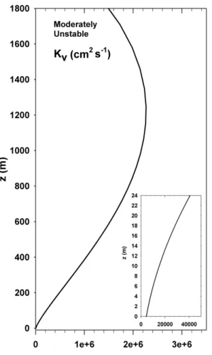
In the PBL above the canopy, the parameterization of Ulke (2000) is used

Kv(z)=0.4u∗h

z

h 1−

z h

g

z,h

L

(33)

wheregis a function of atmospheric stability,

g=

1+6.9h

L z h

−1

for stable conditions, h

L >0 (34)

5

g=

1−22h

L z h

1/4

for unstable conditions, h

L <0 (35)

g=1 for neutral conditions, h

L =0 (36)

At canopy top, the Ulke (2000) and Raupach (1989a) eddy diffusivities are matched by adjusting the value ofα1as a function ofh/L(withα0=0.45,α1ranges over 0.5–2.0

10

as a function of atmospheric stability).

2.5 Background mixing

ACCESS includes an optional process to account for the influence of background sources of trace species on chemistry within and above the canopy. Mixing from these background sources is represented by

15

Ai(z)=−kb

Ci(z)−Cb_i

(37)

where,kb is an adjustable mixing rate (s

−1

) and Cb_i are prescribed background trace species concentrations. This process is configured so that it can be applied to either

(19)

ACPD

12, 24765–24820, 2012

R. D. Saylor

Title Page

Tables Figures

◭ ◮

Back Close

Full Screen / Esc

Discussion

P

a

per

|

Dis

cussion

P

a

per

|

Discussion

P

a

per

|

Discussio

n

P

a

per

|

all integrated species or to only a selected subset. When applied to all species, it sim-ulates a true advective mixing process of air from an upwind source, but when applied to only a selected subset of species, it acts to constrain the selected species to tend towards the prescribed values. In this way, simulations can be run where species mea-sured in a field campaign can be constrained to observed values or the background 5

values of certain selected species can be varied to investigate their impact on chem-ical processes within the canopy. For the simulations reported here, a subset of CH4,

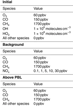
CO and O₃were prescribed at 1700, 150 and 60 ppbv, respectively, with a mixing rate time constant of∼3 h. Additionally, in the experiments presented in Sect. 4, NOx

back-ground values were prescribed across a range of 0.1–30 ppbv to investigate the impact 10

of anthropogenic NO_xsources on canopy biogenic hydrocarbon fluxes.

3 Application to an isoprene-emission-dominated deciduous forest

The Walker Branch Watershed (WBW) is a dedicated ecosystem research area on the US Department of Energy’s Oak Ridge Reservation in east Tennessee. The 97.5 ha watershed has been the site of long-term ecosystem and atmospheric research ac-15

tivities since the mid-1960s. A flux tower located within the watershed (35◦57′30′′N, 84◦17′15′′W; 365 m above mean sea level) and 10 km southwest of Oak Ridge, Ten-nessee, has served as a focal point for previous atmospheric turbulence and chemical flux measurements (Baldocchi et al., 1984, 1995, 1999; Harley et al., 1997; Fuentes et al., 2007) and the canopy morphology of the forest surrounding the flux tower has 20

been extensively documented (Hutchison et al., 1986; Baldocchi and Hutchison, 1986; Baldocchi et al., 2002). The forest is mixed deciduous consisting of chestnut oak (Quer-cus prinus), tulip poplar (Liriodendron tulipifera), white oak (Quer(Quer-cus alba), red oak (Quercus rubra), red maple (Acer rubrum), and various hickory species (Carya sp.) in order of decreasing biomass density (Kardol et al., 2010). Since different tree species 25

have differing basal isoprene emission rates (Geron et al., 2001), the effective leaf-level isoprene emission rate,E_bisop, is dependent on the composition and prevalence of tree

(20)

ACPD

12, 24765–24820, 2012

R. D. Saylor

Title Page

Tables Figures

◭ ◮

Back Close

Full Screen / Esc

Discussion

P

a

per

|

Dis

cussion

P

a

per

|

Discussion

P

a

per

|

Discussio

n

P

a

per

|

species and their biomass density in the forest canopy being simulated. In this study, a value ofE_bisop was chosen to be consistent with canopy-scale isoprene fluxes mea-sured at the WBW flux tower. At the time of isoprene flux measurements made at the tower (Baldocchi et al., 1995, 1999; Fuentes et al., 2007), the stand was approximately 50 yr old, the overstory canopy height (h_c) was 24 m, and the whole canopy leaf area 5

index (LAI) was 4.9 m2leaf m−2 ground area. In this work, ACCESS was applied to the WBW forest to investigate the influence of background anthropogenic NOxsources

on above canopy fluxes of SOA precursors in an isoprene-emission-dominated land-scape. The modeled leaf area density (LAD) function of the canopy (idealized from the measurements of Hutchison et al., 1986) is shown in Fig. 1.

10

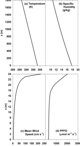
Although ACCESS has been designed to ingest meteorological and radiative flux data from a variety of sources, including vertically resolved land surface models or canopy environment models, in this work a combination of climatological data and em-pirical parameterizations were used to generate input data for the WBW forest appli-cation (Figs. 2, 3). ACCESS was run in steady-state mode, simulating 02:00 p.m. LT 15

on 10 July, with a surface temperature of 303 K with a vertical profile determined by a 6.5 K km−1lapse rate, surface pressure of 970 mb (geopotential pressure correspond-ing to 365 m ASL), and 60 % relative humidity. Above canopy solar insolation,E0, was

computed for clear sky conditions from the empirical formulation of Meyers and Dale (1983) and canopy top PPFD was then approximated as 0.49E0 and converted to

20

µmol photons m−2s−1. Attenuation of PPFD or actinic flux within the forest canopy is formulated as

I(z)=I0·exp (−κf·LAIΣ(z)) (38)

where,κfis the canopy attenuation function for WBW forest as described by Baldocchi

and Hutchison (1986) and LAI_Σis the top-down cumulative leaf area index (m2m−2) of 25

the canopy computed from the leaf area density profile. Finally, the mean wind speed

(21)

ACPD

12, 24765–24820, 2012

R. D. Saylor

Title Page

Tables Figures

◭ ◮

Back Close

Full Screen / Esc

Discussion

P

a

per

|

Dis

cussion

P

a

per

|

Discussion

P

a

per

|

Discussio

n

P

a

per

|

within the canopy, ¯u(z), is computed from the empirical relation of Meyers et al. (1998)

¯

u(z)=u¯(hc) exp

−γLAI 1−z/hc

β

(39)

where, ¯u(hc) is the mean wind speed at canopy top,γLAIis the whole canopy LAI (with

a maximum value of 4), andβis a canopy specific empirical parameter that is set equal to 0.5 for typical deciduous forests.

5

4 Results and discussion

The gas phase oxidation of monoterpenes and sesquiterpenes was originally thought to be the only pathway that produced significant amounts of biogenically derived SOA. However, recently many studies have suggested that additional pathways exist for SOA formation, including gas-phase isoprene reactions (Claeys et al., 2004; Kroll et al., 10

2006) and aqueous-phase processing of soluble oxidation products of both isoprene and terpenes (Hallquist et al. 2009; Ervens, et al., 2008; Lim et al., 2010). In the SE USA, isoprene emissions dominate biogenic hydrocarbon sources, accounting for more than 80 % of total BVOC emissions (Goldstein et al., 2009). Organic matter (OM) com-prises roughly 30–40 % of total fine particle mass in the SE USA (Edgerton et al., 15

2005; Tanner and Parkhurst, 2000) and evidence has accumulated that isoprene oxi-dation products are routinely found in PM_2.5 samples from this region (Clements and Seinfeld, 2007; Edney et al., 2005). Furthermore,14C isotope studies have indicated that the majority of organic matter in fine particles over the entire USA originates from modern sources rather than fossil ones (Schichtel et al., 2008) and this is true in the 20

SE USA as well (Tanner et al., 2004; Ding et al., 2008b; Lee et al., 2010). As a whole, this evidence strongly suggests that SOA formed from biogenic isoprene emissions contributes significantly to total fine particle OM in the SE USA.

However, as summarized by Lee et al. (2010), there is substantial evidence of a strong anthropogenic influence on OM concentrations in the SE USA, in particular for 25

(22)

ACPD

12, 24765–24820, 2012

R. D. Saylor

Title Page

Tables Figures

◭ ◮

Back Close

Full Screen / Esc

Discussion

P

a

per

|

Dis

cussion

P

a

per

|

Discussion

P

a

per

|

Discussio

n

P

a

per

|

measurements of water-soluble organic carbon (WSOC) in PM_2.5(Weber et al., 2007; Sullivan and Weber, 2006; Zhang et al., 2012), which exhibit strong correlations with anthropogenic pollutants such as CO, elemental carbon and fossil fuel hydrocarbons. On the other hand, Ding et al. (2008a) observed significant correlations of WSOC from PM2.5 samples in the SE USA with the isoprene oxidation products 2-methyltetrols.

5

Weber et al. (2007) speculate that some anthropogenic component (or components) influences the amount of SOA formed, regardless of whether the VOC is biogenic or anthropogenic in origin. In a comprehensive review article, Hoyle et al. (2011) sur-vey the currently known possible mechanisms through which anthropogenic sources may enhance the formation of biogenic SOA. In this work, ACCESS is applied to an 10

isoprene-emission-dominated forest canopy to investigate the relative magnitude of SOA precursor concentrations and fluxes above the canopy as a function of back-ground levels of NOx. Assuming that higher levels of background NOx are associated

with anthropogenic sources, the results of these simulations may suggest one mech-anism by which higher levels of biogenic SOA can be directly correlated with anthro-15

pogenic influences.

Although details of the mechanism of isoprene oxidation are still the subject of vigor-ous investigation and some uncertainty (Stone et al., 2011; Archibald et al., 2010a,b; Galloway et al., 2011), in particular the apparent shortcomings of HOxchemistry in low

NO_x, high isoprene environments (Lelieveld et al., 2008; Hofzumahaus et al., 2009; 20

Pugh et al., 2010), the broad outlines of first- and second-generation products from isoprene oxidation are relatively well defined. Carlton et al. (2009) reviewed current understanding of the reaction pathways that may lead to SOA formation from iso-prene. First-generation products methacrolein and methyl vinyl ketone (MVK) are the best characterized and evidence indicates that reactions involving methacrolein likely 25

lead to SOA formation while MVK reaction products do not. Under low NO_x condi-tions, first-generation organic peroxides are more prevalent (Surratt et al., 2006), but as previously mentioned there is substantial mechanistic uncertainty in this regime. Considerable interest has recently been focused on several small, second-generation

(23)

ACPD

12, 24765–24820, 2012

R. D. Saylor

Title Page

Tables Figures

◭ ◮

Back Close

Full Screen / Esc

Discussion

P

a

per

|

Dis

cussion

P

a

per

|

Discussion

P

a

per

|

Discussio

n

P

a

per

|

products including glyoxal, glycolaldehyde, methyl glyoxal and hydroxyacetone. Ab-sorption and chemical processing of these water-soluble compounds in cloud droplets or wet aerosols are suspected to add to total SOA mass via aqueous oligomeriza-tion reacoligomeriza-tions (Lim et al., 2005; Ervens et al., 2008; Altieri et al., 2006, 2008; Carlton et al., 2007; Ortiz-Montalvo et al., 2012). Recent global-scale simulations including 5

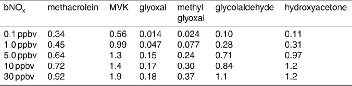
aqueous-phase SOA production have indicated that these pathways account for a sub-stantial fraction of total SOA produced in the global atmosphere (Liu et al., 2012; Lin et al., 2012). In the simulations reported below, the concentration profiles and fluxes of methacrolein, MVK, glyoxal, methyl glyoxal, glycolaldehyde and hydroxyacetone are examined as a function of background NOxlevels.

10

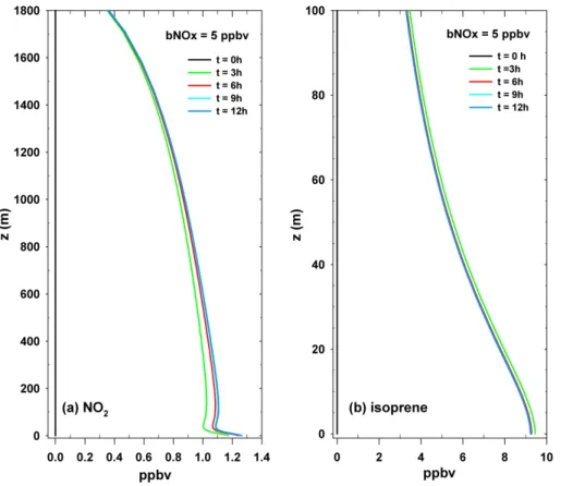
For each experiment of the simulated WBW canopy, a fixed concentration of NO_x (0.1, 1.0, 5, 10 and 30 ppbv) was specified for a well-mixed background boundary layer that was mixed into the column with a∼3 h mixing time constant (Wolfe and Thorn-ton, 2011). Each simulation was run with fixed vertical profiles of all meteorological (Figs. 2, 3) and isoprene emissions data (Fig. 4) and a fixed solar zenith angle corre-15

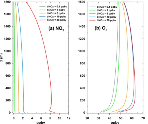
sponding to 02:00 p.m. LT at the WBW latitude and longitude. Initial conditions, back-ground concentrations and free tropospheric concentrations were identical for each simulation as specified in Table 1. The simulations were each run for a total of 12 h which allowed ample time for a steady state to be achieved for all species, as shown in Fig. 5 for NO₂ and isoprene. All results shown below use profiles fromt=12 h as the 20

steady-state result. Figure 6 presents the steady-state profiles of NO₂ and O₃ which resulted for each specified background NOx(bNOx) value.

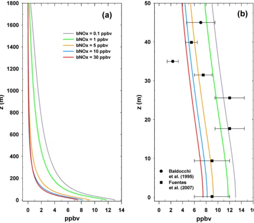
Simulated vertical profiles of isoprene as a function of background NOxvalue are

pre-sented in Fig. 7. Profiles over the full model domain (Fig. 7a) exhibit a relatively rapid monotonic decrease with height as is expected for a near surface emitted species that 25

is chemically reactive. Increasing bNOx values increase the reactivity of the system,

thereby decreasing the steady-state values of isoprene throughout the modeled col-umn. Modeled isoprene mixing ratios in and just above the canopy (Fig. 7b) are seen to agree relatively well with measurements (means ±1 standard deviation) made by

(24)

ACPD

12, 24765–24820, 2012

R. D. Saylor

Title Page

Tables Figures

◭ ◮

Back Close

Full Screen / Esc

Discussion

P

a

per

|

Dis

cussion

P

a

per

|

Discussion

P

a

per

|

Discussio

n

P

a

per

|

Baldocchi et al. (1995) and Fuentes et al. (2007) at the WBW flux tower. The modeled near-surface mixing ratios and vertical profiles also compare favorably with other profile measurements made in or near the SE USA. Andronache et al. (1994) analyzed ver-tical profiles of isoprene from balloon-borne measurements made in western Alabama during July 1990 and found means of 37 profiles which ranged from >4 ppbv at the 5

surface and dropped quickly to less than 2 ppbv by 300 m above ground level (AGL). They categorized the profiles into two groups roughly equal in number, “simple” profiles in which the mixing ratio decreased monotonically with height and “complex” profiles where a maximum occurred somewhere above the surface. The “complex” profiles were characterized by non-uniform turbulence structures with layers of strong wind 10

shear or enhanced vertical stability. Wiedinmyer et al. (2005) presented surface and balloon-borne isoprene measurements made in and near the Ozarks in central Mis-souri as part of the Ozarks Isoprene Experiment in July 1998. Ground-level isoprene mixing ratios ranged from<1 to 35 ppbv in the oak dominated forests of the Ozarks (similar to WBW) and balloon-measured means of afternoon mixing ratios ranged from 15

3–4 ppbv near 200 m AGL to<2 ppbv just above 800 m AGL.

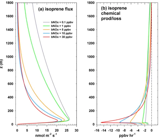
Modeled vertical fluxes of isoprene (Fig. 8a) peak near 50–70 m, whereas the maximum chemical loss of isoprene (Fig. 8b) occurs just above the canopy top (∼30 m) where maximum photochemical activity occurs. As seen in Fig. 8, as bNOx

in-creases over the simulated range, peak chemical loss rates of isoprene increase from 20

<2 ppbv h−1 to almost 15 ppbv h−1 just above canopy top, while the maximum iso-prene flux decreases from>26 to near 20 nmol m−2s−1(a decrease of>20 %). Maxi-mum modeled isoprene fluxes at or just above canopy top were also observed by Gao et al. (1993) and Doskey and Gao (1999). Stroud et al. (2005) examined the impact of anthropogenic pollution on the overall canopy fluxes of isoprene and only found a small 25

change (a maximum 4 % decrease) between scenarios ranging from clean continental to urban. Results from other canopy modeling efforts have varied widely in assess-ing the impact that chemical loss has on isoprene fluxes from the canopy. Usassess-ing the same base model as Stroud et al. (2005), Makar et al. (1999) estimated that neglecting

(25)

ACPD

12, 24765–24820, 2012

R. D. Saylor

Title Page

Tables Figures

◭ ◮

Back Close

Full Screen / Esc

Discussion

P

a

per

|

Dis

cussion

P

a

per

|

Discussion

P

a

per

|

Discussio

n

P

a

per

|

chemistry would result in substantially (∼40 %) larger isoprene mixing ratios above the canopy. On the other hand, Gao et al. (1993) and Doskey and Gao (1999) both esti-mated only negligible impact of chemical loss on above canopy isoprene fluxes, while Forkel et al. (2006) reported a 10–15 % reduction in isoprene fluxes due to chemistry. Because these studies use various condensed chemical mechanisms and have at-5

tempted to simulate different forest canopy morphologies and species across a broad range of BVOC emission rates and background chemical concentrations, it is difficult to draw definitive conclusions. Reconciling these disparate results will require a more complete investigation into the environmental, biological and anthropogenic factors that may influence the role that chemistry plays in above canopy isoprene fluxes.

10

Fuentes et al. (2007) presented data from one day (20 July) at WBW showing that isoprene measurements peaked in the upper levels of the canopy, however model re-sults from ACCESS exhibit a gradual decrease of isoprene from the surface upwards, which is typical for a relatively well-mixed vertical column. To obtain peaks in isoprene at canopy top that are 30 % larger than values obtained at or near the surface as shown 15

by Fuentes et al. (2007) may imply only very slight vertical mixing when these measure-ments were taken, since it would not be expected that chemical loss of isoprene would be stronger deeper within the shaded canopy. However, since Fuentes et al. (2007) do not provide details concerning in-canopy turbulence or atmospheric stability (other than modeled canopy residence times) on the day of these measurements, it is diffi -20

cult to assess this supposition. As mentioned earlier, it has been recognized for some time that within canopy turbulence is complex; several recent studies (Steiner et al., 2011; Bryan et al., 2012; Dupont and Patton, 2012) have re-emphasized the impor-tance of simultaneous measurement of turbulent mixing parameters when performing chemical profile measurements in and above forest canopies. The frequency of oc-25

currence (roughly half of the total measurements) of the “complex” vertical profiles of Andronache et al. (1994) also emphasizes the importance of detailed characterization of the atmospheric turbulence structure within and above the canopy for a full under-standing of chemically reactive exchanges between the biosphere and atmosphere.

(26)

ACPD

12, 24765–24820, 2012

R. D. Saylor

Title Page

Tables Figures

◭ ◮

Back Close

Full Screen / Esc

Discussion

P

a

per

|

Dis

cussion

P

a

per

|

Discussion

P

a

per

|

Discussio

n

P

a

per

|

Simulated mixing ratio profiles, vertical fluxes and chemical production/loss rates are presented as a function of bNOx for first- and second-generation products of

iso-prene oxidation in Figs. 9–14. The first generation products methacrolein (Fig. 9) and MVK (Fig. 10) exhibit similar profiles, with MVK concentrations and fluxes generally being larger (roughly 2×) for a given bNOx value. The peaks of chemical production

5

of methacrolein and MVK coincide with the maximum chemical loss of isoprene just above canopy top (∼30 m) and the magnitude of chemical production increases with increasing bNOxvalue. Higher in the boundary layer, the net chemical budget for these

species changes from production to loss as conversion to second-generation products becomes more dominant than production from isoprene. The height above canopy top 10

where this transition from net production to net loss occurs decreases with increasing bNOxvalue, as does the height of maximum vertical flux.

The second-generation products glyoxal (Fig. 11), methyl glyoxal (Fig. 12), glyco-laldehyde (Fig. 13), and hydroxyacetone (Fig. 14) exhibit vertical profiles and variations with bNOxthat are similar to each other but different from methacrolein and MVK.

Mix-15

ing ratio vertical profiles of the second-generation products do not drop offin magnitude with height as quickly as with methacrolein and MVK and vertical flux profiles generally continue to increase throughout the depth of the boundary layer for all values of bNOx.

Additionally, the vertical profile of the chemical production rate of second-generation products changes significantly with increasing bNO_xand the height at which the peak 20

rate occurs lowers with increasing bNOx values. It is notable that the magnitudes of

the vertical profiles of these species do not necessarily increase monotonically with in-creases in bNO_x value but exhibit inherent non-linearities. For example, the glyoxal mixing ratio for bNOx =30 ppbv is larger near the surface than the value at bNOx =10 ppbv, but eventually decreases below the profiles for both bNOx =10 ppbv and

25

bNO_x ₌5 ppbv above 400 m. Similarly, the vertical profiles (and fluxes) of methyl gly-oxal, glycolaldehyde and hydroxyacetone exhibit non-linear variations with bNOx that

are non-intuitive, reflecting a complex interaction between vertical transport and chem-istry. For second-generation products shown in Figs. 11–14, the relative magnitude of