www.atmos-chem-phys.net/16/15461/2016/ doi:10.5194/acp-16-15461-2016
© Author(s) 2016. CC Attribution 3.0 License.
Modelling bidirectional fluxes of methanol and acetaldehyde
with the FORCAsT canopy exchange model
Kirsti Ashworth1,a, Serena H. Chung2, Karena A. McKinney3,b, Ying Liu3,b,c, J. William Munger3,4, Scot T. Martin4, and Allison L. Steiner1
1Climate and Space Science and Engineering, University of Michigan, Ann Arbor, MI 48109, USA
2Department of Civil and Environmental Engineering, Washington State University, Pullman, WA 99164, USA 3Department of Earth and Planetary Sciences, Harvard University, Cambridge, MA 02138, USA
4School of Engineering and Applied Sciences, Harvard University, Cambridge, MA 02138, USA
anow at: Royal Society Dorothy Hodgkin Research Fellow at Lancaster Environment Centre, Lancaster University,
LA1 4YQ, UK
bformerly at: of Department of Chemistry, Amherst College, Amherst, MA 01002, USA cnow at: Peking University, Beijing 100000, China
Correspondence to:Kirsti Ashworth ([email protected])
Received: 16 June 2016 – Published in Atmos. Chem. Phys. Discuss.: 30 June 2016
Revised: 27 November 2016 – Accepted: 28 November 2016 – Published: 15 December 2016
Abstract.The FORCAsT canopy exchange model was used to investigate the underlying mechanisms governing foliage emissions of methanol and acetaldehyde, two short chain oxygenated volatile organic compounds ubiquitous in the tro-posphere and known to have strong biogenic sources, at a northern mid-latitude forest site. The explicit representation of the vegetation canopy within the model allowed us to test the hypothesis that stomatal conductance regulates emissions of these compounds to an extent that its influence is observ-able at the ecosystem scale, a process not currently consid-ered in regional- or global-scale atmospheric chemistry mod-els.
We found that FORCAsT could only reproduce the magni-tude and diurnal profiles of methanol and acetaldehyde fluxes measured at the top of the forest canopy at Harvard Forest if light-dependent emissions were introduced to the model. With the inclusion of such emissions, FORCAsT was able to successfully simulate the observed bidirectional exchange of methanol and acetaldehyde. Although we found evidence that stomatal conductance influences methanol fluxes and concentrations at scales beyond the leaf level, particularly at dawn and dusk, we were able to adequately capture ecosys-tem exchange without the addition of stomatal control to the standard parameterisations of foliage emissions, suggesting
that ecosystem fluxes can be well enough represented by the emissions models currently used.
1 Introduction
in-clude dynamic biogenic sources and sinks of oVOCs. While most now incorporate online calculations of biogenic emis-sions of isoprene and monoterpenes, based on the light and temperature-dependence algorithms developed by Guenther et al. (1995, 2006, 2012), methanol emissions have only been recently included in some CTMs (e.g. GEOS-Chem, Millet et al., 2010; Laboratoire de Météorologie Dynamique zoom (LMDz), Folberth et al., 2006), and most still rely on non-dynamic emissions inventories for methanol and acetalde-hyde if primary biogenic emissions of these species are in-cluded (e.g. UKCA; O’Connor et al., 2014). Furthermore, Ganzeveld et al. (2008) demonstrated the weaknesses of the algorithms currently used in 3-D chemistry transport mod-els to calculate primary emissions of methanol online. Simi-larly, dry deposition schemes in CTMs are usually based on fixed deposition velocities (Wohlfahrt et al., 2015) or calcu-lated from roughness lengths and leaf area index values as-signed to generic land cover types (e.g. FRSGC-UCI, Wild et al., 2014; LMDz, Folberth et al., 2006). This simplistic ap-proach to biogenic sources and sinks may be a critical omis-sion limiting their capability of accurately simulating atmo-spheric composition in many world regions.
Here we focus on methanol and acetaldehyde, two oVOCs that are frequently observed in and above forests but whose sources, sinks, and net budgets are not known with any cer-tainty (Seco et al., 2007; Niinemets et al., 2004). While bio-genic sources of both are strongly seasonal, fluxes and con-centrations can remain high throughout the growing season (Stavrakou et al., 2011; Millet et al., 2010; Hu et al., 2011; Karl et al., 2003; Wohlfahrt et al., 2015). Methanol fluxes are on the same order of magnitude as isoprene at many sites in the US (Fall and Benson, 1996), suggesting their regional and global importance. The fundamental mechanisms lead-ing to the synthesis and/or subsequent release of methanol and acetaldehyde are not currently fully understood (Karl et al., 2002; Seco et al., 2007).
Methanol is known to be produced from demethylation processes during cell wall expansion and leaf growth with emissions peaking during springtime leaf growth and declin-ing with leaf age (Fall and Benson, 1996). The factors con-trolling the subsequent release of methanol to the atmosphere are harder to decipher (Huve et al., 2007; Niinemets et al., 2004). Measurements at all scales, from leaf-level to branch-enclosure and ground-based ecosystem-scale field measure-ments (e.g. Kesselmeier, 2001; Kesselmeier et al., 1997; Karl et al., 2003; Seco et al., 2015; Wohlfahrt et al., 2015), as well as satellite inversions (e.g. Stravakou et al., 2011) demon-strate a strong diurnal profile of methanol fluxes similar to that of isoprene (e.g. Fall and Benson, 1996). Methanol syn-thesis, unlike that of isoprene, is not specifically linked to photosynthesis and the light dependence observed in leaf-level emissions have been shown to result from regulation by the stomata due to the high solubility of methanol in water (e.g. Nemecek-Marshall et al., 1995; Niinemets and Reich-stein, 2003a, b; Huve et al., 2007).
The pathways leading to both the synthesis and emission of acetaldehyde are not clear (Karl et al., 2002; Jardine et al., 2008). Acetaldehyde has long been known to be an oxidation product of ethanol produced in leaves under anoxic condi-tions (Kreuzwieser et al., 2000), but this cannot explain the strong emissions observed under normal environmental con-ditions in mid-latitude forests (e.g. Seco et al., 2007; Karl et al., 2003). Karl et al. (2003) observed that bursts of ac-etaldehyde were emitted during light–dark transitions and postulated that such emissions were associated with pyru-vate decarboxylation. Leaf-level measurements of acetalde-hyde emissions have also been found to be tightly coupled to stomatal aperture (e.g. Kreuzwieser et al., 2000; Karl et al., 2002; Niinemets et al., 2004), and it has been suggested that this may account for observed light-dependent ecosystem-scale emissions of acetaldehyde (Jardine et al., 2008).
Previous studies have suggested that the role of stomatal conductance in determining net flux of oVOCs could be in-corporated in large-scale models by adopting a compensa-tion point approach (see e.g. Harley et al., 2007; Ganzeveld et al., 2008; Jardine et al., 2008). The compensation point for a given compound is the atmospheric concentration of that compound at which the leaf, plant, or canopy switches from acting as a net source to a net sink. While firmly based in plant physiology and plant response to environmental con-ditions, this approach would allow models lacking leaf-level processes to account for the changes in flux direction (Harley et al., 2007; Ganzeveld et al., 2008). Observational (Jardine et al., 2008) and modelling studies (Ganzeveld et al., 2008) have both shown the potential power of this approach, al-though Jardine et al. (2008) found that the compensation point was heavily dependent on light and temperature and may therefore not be straightforward to implement.
emis-sions and with fluxes measured just above the top of the canopy at Harvard Forest in July 2012.
2 Methods
2.1 Harvard Forest measurements
Harvard Forest is situated in a rural area of Massachusetts, approximately 90 km from Boston and 130 km from Al-bany. It is classified as a mixed deciduous broadleaved for-est, with red oak (36 %) and red maple (22 %) as the dom-inant species (Urbanski et al., 2007). Continuous measure-ments of micrometeorological variables and air pollutants have been made from the Environmental Monitoring Station (EMS) Tower, part of the AmeriFlux network, for 25 years (Urbanski et al., 2007; Munger and Wofsy, 1999a, b). The tower, located at 42.5◦N and 72.2◦W and an elevation of 340 m, is 30 m high and is surrounded by primary forest with an average height of around 23 m. The long-term meteoro-logical measurements include photosynthetically active ra-diation (PAR), relative humidity (RH), and air temperature at multiple heights on the tower, together with wind speed and direction recorded just below the top of the tower (at
∼29 m; Urbanski et al., 2007; Munger and Wofsy, 1999a). In addition to exchanges of CO2 collected to assess
photo-synthetic activity and productivity, concentrations of CO at the top of the tower and fluxes of O3(at multiple heights on
the tower) are also routinely measured (Munger and Wofsy, 1999c). NO and NO2 concentrations and fluxes have been
recorded in the past (Munger et al., 1996, 1998), with the most recent measurements in 2002 (Horii et al., 2004). In ad-dition to these continuous atmospheric measurements, a suite of other data are gathered periodically to determine ecosys-tem health and functioning. Such data include leaf area in-dex, tree girth, litter mass, leaf chemistry, and soil moisture and respiration (Barford et al., 2001; Urbanski et al., 2007; Munger and Wofsy, 1999b).
Concentrations and fluxes of bVOCs and their oxidation products have also been measured at the EMS Tower dur-ing several summer growdur-ing seasons (McKinney et al., 2011; Goldstein et al., 1998, 1995), augmenting the AmeriFlux suite of observations. Between 7 June and 24 September 2012, a proton-transfer-reaction time-of-flight mass spec-trometer (PTR-TOF-MS 8000, Ionicon Analytik GmbH, Austria) was used to measure the concentrations of volatile organic compounds at the site. The PTR-TOF-MS is capable of rapidly detecting hundreds of different VOCs at concen-trations as low as a few pptv. PTR-TOF-MS has been pre-viously described by Jordan et al. (2009a, b) and Graus et al. (2010). The instrument utilises a high-resolution TOF de-tector (Tofwerk AG, Switzerland) to analyse the reagent and product ions and allows for exact identification of the ion molecular formula (mass resolution > 4000).
Ambient air was sampled from an inlet mounted at the top of the 30 m EMS Tower at a total flow rate of 5 slpm us-ing a configuration identical to that used by McKinney et al. (2011) in 2007. H3O+ reagent ions were used to
selec-tively ionise organic molecules in the sample air. The in-strument was operated with a drift tube temperature of 60◦C and a drift tube pressure of 2.20 mbar. The drift tube voltage was set to 550 V, resulting in anE/N of 126 Td (E, electric field strength;N, number density of air in the drift tube; unit, Townsend, Td; 1 Td=10−17V cm2). PTR-TOF-MS spectra
were collected at a time resolution of 5 Hz. Mass calibra-tion was performed every 2 min with data acquisicalibra-tion using the Tof-Daq v1.91 software (Tofwerk AG, Switzerland). A calibration system in which gas standards (Scott Specialty Gases) were added into a humidified zero air flow at con-trolled flow rates was used to establish the instrument sen-sitivities to VOCs. Every 3 h the inlet flow was switched to pass through a catalytic converter (platinum on glass wool heated to 350◦C) to remove VOCs and establish background intensities.
The PTR-TOF-MS captures the entire mass spectrum in each 5 Hz measurement, providing a continuous mixing ratio time series at each mass-to-charge ratio rather than the dis-junct time series obtained in previous PTR-MS studies at this site (McKinney et al., 2011). As a result, direct, rather than virtual disjunct, eddy covariances were determined and are reported herein (Mueller et al., 2010). Wind speeds recorded at 8 Hz by a tridimensional sonic anemometer located at the same height and less than 1 m away from the gas inlet were averaged to a 5 Hz time base, synchronised with the mixing ratio data, and used in the eddy covariance calculations. Eddy covariance fluxes were calculated from the data for 30 min intervals using methods described in McKinney et al. (2011). Ambient mixing ratios were averaged over the same 30 min intervals for which fluxes were calculated. The 30 min aver-age mixing ratios and fluxes were then binned by time of day to calculate diurnal averages.
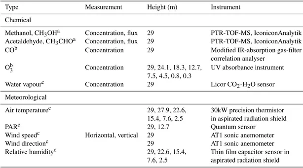
Table 1.Atmospheric and meteorological measurements relevant to this study made between 7 June and 24 September 2012 at the EMS Tower in Harvard Forest.
Type Measurement Height (m) Instrument
Chemical
Methanol, CH3OHa Concentration, flux 29 PTR-TOF-MS, IconiconAnalytik
Acetaldehyde, CH3CHOa Concentration, flux 29 PTR-TOF-MS, IconiconAnalytik COb Concentration 29 Modified IR-absorption gas-filter
correlation analyser Ob3 Concentration 29, 24.1, 18.3, 12.7, UV absorbance instrument
7.5, 4.5, 0.8, 0.3
Water vapourc Concentration 29 Licor CO2-H2O sensor
Meteorological
Air temperaturec 29, 27.9, 22.6, 30kW precision thermistor 15.4, 7.6, 2.5 in aspirated radiation shield
PARc 29, 12.7 Quantum sensor
Wind speedc Horizontal, vertical 29 AT1 sonic anemometer
Wind directionc 29 AT1 sonic anemometer
Relative humidityc 29, 22.6, 15.4, Thin film capacitor sensor in 7.6, 2.5 aspirated radiation shield
aData provided by McKinney and Liu.bMunger and Wofsy (1999b).cMunger and Wofsy (1999a).
correlated, suggesting no systematic bias in the application of eddy covariance at this site.
Isoprene, total combined monoterpenes, MVK (methyl vinyl ketone) and MACR (methacrolein) (detected as a sin-gle combined species), methanol, acetaldehyde, and acetone were all detected at concentrations well above the PTR-MS detection limit and determined to be free from interference from other compounds (McKinney et al., 2011). Here we confine our analysis to concentrations and fluxes of methanol and acetaldehyde. Table 1 summarises the relevant flux, con-centration, and meteorological measurements made at the EMS Tower during the summer of 2012.
2.2 FORCAsT1.0 canopy exchange model
FORCAsT (version 1.0) is a single column (1-D) model that simulates the exchange of trace gases and aerosols between the forest canopy and atmosphere. A full description of FOR-CAsT is given in Ashworth et al. (2015). Here we provide a brief overview, summarise biogenic emissions and flux calculations in the model and describe the simulations per-formed.
FORCAsT1.0 has 40 vertical levels of varying thickness extending to a height of ∼4 km, with the highest
resolu-tion nearest the ground where the complexity is greatest, i.e. within the canopy space. Micrometeorological conditions (temperature, PAR, RH) within the canopy are determined prognostically by energy balance, accounting for the physi-cal structure of the canopy. The gas-phase chemistry scheme incorporated in FORCAsT1.0 is a modified version of the CalTech Chemical Mechanism (CACM; Griffin et al., 2002,
2005; Chen and Griffin, 2005), which includes 300 species whose concentrations are solved at every chemistry timestep (currently 1 min), plus O2and water vapour (Ashworth et al.,
2015). Of the species, 99 are assumed to be condensable, and are lumped into 11 surrogate groups based on similar volatil-ity and structure. Aerosol-phase concentrations of these sur-rogate groups are also calculated at every timestep based on equilibrium partitioning (Ashworth et al., 2015; Chen and Griffin, 2005).
The CACM chemistry mechanism in FORCAsT treats methanol explicitly with no chemical sources (e.g., produc-tion from peroxy radicals) and a sink via oxidaproduc-tion by OH to produce formaldehyde. Acetaldehyde is not treated explic-itly but is instead included in a lumped group of aldehydes (ALD1, with < C5). The oxidation reactions for this group
are based on acetaldehyde and no other species is currently emitted into the ALD1 group. Acetaldehyde has a far greater number of chemical sources and sinks in the FORCAsT sim-ulations of a forest environment than methanol. See Ash-worth et al. (2015) for details of the reactions and reaction rates included in FORCAsT.
Table 2.Boundary and initial conditions used for the FORCAsT simulations.
Model parameter or variable Value
Total leaf area index (m2leaf area m−2ground area)a 3.67
Average canopy height (m)b 23.0 Average trunk height (m)b 6.0
Meteorology (values measured at 29 m)
Air temperature (◦C)c 20.9
Wind speed (m s−1)c 1.589
Friction velocity,u∗(m s−1)d 0.278
Standard deviation of vertical wind velocity,σw(m s−1)d 0.351
Concentrations at 29 m (ppbv)
Isoprenee 0.939
Total monoterpenese 0.449
MVK-MCRe 0.786
Methanole 10.11
Acetaldehydee 0.620
Acetonee 2.608
Ozonef 33.54
COf 164.8
Water vapourc 1.861 %
Miscellaneous
Ozone at ground level (0.3 m)f 20.35 ppbv Temperature at ground level (2.5 m)c 18.1◦C Soil temperature at 15, 40, 50, and 90 cm deptha 24.9, 25.9, 25.9,
21.4◦C Soil moisture at 15, 40, 50, and 90 cm deptha 0.18, 0.15,
0.17, 0.18
NO2at 29 mg 1.00 ppbv
N2O5at 29 mg 1.50 ppbv
aMunger and Wofsy (1999c).bParker (1998).cMunger and Wofsy (1999a).dData provided by
Munger.eData provided by McKinney and Liu.fMunger and Wofsy (1999b).gMunger et al. (1996).
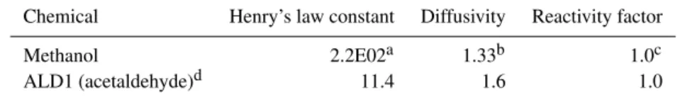
the surface resistance term includes cuticular, mesophyl-lic, and stomatal resistances, which are dependent on the physico-chemical properties of the depositing species as well as the light, temperature, and water potential of the leaf. The deposition scheme described in Ashworth et al. (2015) and Bryan et al. (2012) has been updated to include methanol. The deposition velocity of acetaldehyde is calculated using parameters for the lumped ALD1 group, and the parameters for ALD1 and methanol deposition are shown in Table 3.
While a 1-D model cannot capture horizontal transport, FORCAsT does include a simple parameterisation to account for advection (Bryan et al., 2012; Ashworth et al., 2015). For the simulations here, only advection of NO2is considered,
such that a NO2mixing ratio of 1 ppbv is set just above the
canopy based on average midday (defined as 10:00–17:00 EST) NOxand NOy(total reactive nitrogen species) concen-trations. While nitrogen species were not measured at Har-vard Forest in 2012, concentrations reported from the site by Munger et al. (1996) are extrapolated to 2012 using July
monthly average NOxlevels measured at the nearby US EPA monitoring station at Ware 42.3◦N, 72.3◦W, elevation 312 m (roughly 30 km southwest of the EMS Tower). This scaling accounts for the observed decrease in NOx levels across the region as a result of emission reduction strategies (see e.g. EPA, 2015). All NOxis assumed to be advected as NO2. The
initial concentration of N2O5at 29 m was set to give an
aver-age NOx: NOy ratio of 0.4 (Munger et al., 1996), assuming all residual NOy to be N2O5initially. Lee et al. (2006) also
Table 3.Deposition parameters for methanol and acetaldehyde.
Chemical Henry’s law constant Diffusivity Reactivity factor
Methanol 2.2E02a 1.33b 1.0c
ALD1 (acetaldehyde)d 11.4 1.6 1.0
aSander (1999).bWesely (1989).cKarl et al. (2010).dAshworth et al. (2015).
2.2.1 Flux calculations
Fluxes of gases and particles are calculated to be proportional to both the concentration gradient and the efficiency of ver-tical mixing between adjacent model layers (Eq. 1). Upward fluxes are modelled as positive and occur when the concen-tration of a particular species is higher at a lower height. The flux,Fi(kg m−2s−1)of an individual species,i, between two model levels is given by
Fi= −KH 1Ci
1z, (1)
where KH is the eddy diffusivity (m2s−1), 1Ci the
dif-ference in mass concentrations (kg−1)at the mid-height of
the levels, and 1zthe difference in height (m) between the levels. Eddy diffusivity, concentrations of all gas-phase and aerosol species, and fluxes are calculated at 1 min timesteps. The eddy diffusivity at the instrument height of 29 m is con-strained by observed wind speeds (Bryan et al., 2012).
Vertical mixing is calculated prognostically in the model following Blackadar (1979) and is driven by observed top-of-canopy radiation and wind speed. The within-top-of-canopy wind profile is calculated following Baldocchi (1988). Turbulence and mixing in the canopy space is then modified according to Stroud et al. (2005), with wind speed and eddy diffusivity constrained to observations at the top of the canopy. A full description of the vertical mixing and its impact on concen-tration gradients is described in Bryan et al. (2012).
Modelled fluxes should be viewed as an instantaneous snapshot, both temporally and spatially, as the calculation re-lies heavily on the concentration gradient across an arbitrary boundary level, in this case the instrument height of 29 m. Actual concentration gradients display rapid fluctuations (see e.g. Steiner et al., 2011) due to heterogeneity in emissions (see e.g. Bryan et al., 2015) and chemistry (see e.g. Butler et al., 2008), as well as the occurrence of coherent structures that can result in counter-gradient flow of matter (Steiner et al., 2011 and references therein).
2.2.2 Biogenic emissions
Emissions of VOCs from vegetation can be described as fol-lowing one of two possible routes (Grote and Niinemets, 2008). In the first, the compound is released to the at-mosphere immediately on production (e.g. isoprene). Such emissions are tightly coupled to photosynthesis and are
there-fore dependent on both temperature and light, falling to zero at night. We refer to such emissions as “direct”. In the sec-ond pathway, VOCs are stored in specialist structures within the plant after their production (e.g. monoterpenes). Emis-sions from these storage pools occur by diffusion and are controlled by temperature alone. We term these “storage” emissions. It is thought that emissions of oVOCs are a com-bination of these (“combo”), with a proportion released di-rectly on synthesis and the remaining fraction emitted from storage pools.
Emission rates are calculated in FORCAsT by modifying basal emission factors (rates at standard conditions, usually 30◦C and 1000 µmol m−2s−1of PAR) according to
empir-ical relationships describing their dependence on light and temperature. These modifications (referred to as activity fac-tors) follow the standard parameterisations of Guenther et al. (1995, 2012). For storage emissions, which are modelled as dependent on temperature only, the activity factor is a sim-ple exponential relationship:
γT =e−β(TL−TS), (2)
where γT is the temperature-dependent activity factor for storage emissions,βthe temperature response factor (K−1), TS is 293 K, andTL(K) the leaf temperature (see Guenther
et al., 2012). For further details of the activity factors for di-rect emissions included in FORCAsT the reader is referred to Ashworth et al. (2015) and references therein.
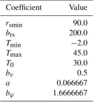
2.3 Stomatal resistance
bal-ance) and deposition rates within FORCAsT. It is not cur-rently used to control the rate of biogenic emissions.
Stomatal resistance is modelled according to leaf tempera-ture, PAR, water potential, and vapour pressure deficit using the relationships developed by Jarvis (1976) as described by Baldocchi et al. (1987). The overall stomatal resistance (rs)
is the product of these individual factors (Eq. 3), which are summarised below in Eqs. (4)–(8).
rs=rsmin·rs(PAR)·rs(T )·rs(D)·rs(p) , (3)
where rs(PAR) is the response of stomatal resistance to
changes in PAR,rsmin(s m−1)is the minimum stomatal
re-sistance, andbrsis an empirical coefficient.
rs(PAR)=rsmin
1+ brs
PAR
(4)
rs(T) is the response of stomatal resistance to changes in leaf temperature (Tlf;◦C),Tmin,Tmax, andT0 are the minimum
and maximum temperatures for stomatal opening and opti-mum temperature respectively:
rs(T )= (
T
lf−Tmin
T0−Tmin
Tmax−Tlf
Tmax−T0 bT)−1
, (5)
bT =
T
max−T0
Tmax−Tmin
. (6)
rs(d) is the relationship between stomatal resistance and
vapour pressure deficit (D; mbar), andbvis an empirical
co-efficient:
rs(D)=
1+bv
D
−1
. (7)
Water potential is assumed to act only once a threshold value is reached. Above this value it is modelled as
rs(ϕ)=
1
a·ϕ+bw
, (8)
whereϕ is the water potential (bar) anda andbw are con-stants. Below the water potential threshold,rs(ϕ) is taken as
unity. The values of the constants used in these calculations are shown in Table 4.
Stomatal resistance is only calculated in FORCAsT during the day (defined within FORCAsT as PAR≥0.01 W m−2); at night stomatal resistance is assumed equal to the minimum cuticular resistance (3000 s m−1).
2.4 FORCAsT simulations
All model simulations were performed for an average day in July 2012, the middle of the growing season, to ensure that measurement data did not include either the spring burst of methanol or elevated acetaldehyde emissions during senes-cence. FORCAsT was initiated with site-specific parameters
Table 4.Values of stomatal resistance coefficients and parameters used in FORCAsT.
Coefficient Value
rsmin 90.0
brs 200.0
Tmin −2.0
Tmax 45.0
T0 30.0
bv 0.5
a 0.066667
bϕ 1.6666667
and measurements of the physical structure of the canopy and environmental conditions (Table 2). Initial meteorolog-ical conditions and atmospheric concentrations of chemmeteorolog-ical species were taken from the 2012 EMS Tower data (see Table 2). Initial air temperature above the canopy is calcu-lated online using the average lapse rate observed by the ra-diosonde at Albany (the nearest sounding station,∼90 km from Harvard Forest) and within the canopy by interpola-tion with the 2 m temperature reading. Concentrainterpola-tions of O3
within the canopy are based on observations from the EMS Tower, and concentrations above the canopy follow a typical night-time profile as described in Forkel et al. (2006). Con-centrations of other species are assumed to decay exponen-tially with height such that thee-folding height is 100m for short-lived species and 1000 m for longer-lived compounds. All model simulations started at 00:00 EST and continued for 48 h, with the same driving data used for each 24 h period and analysis confined to the second day to account for model spin-up.
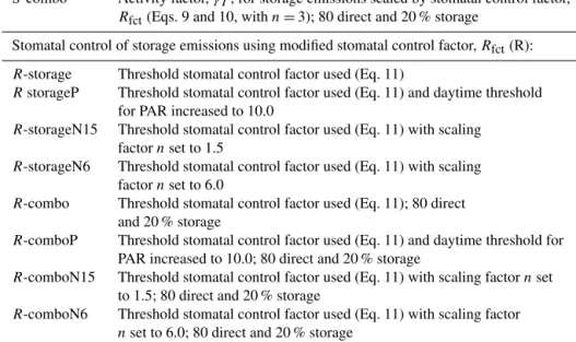
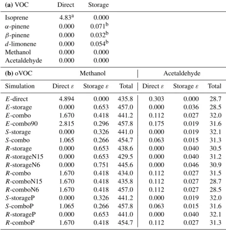
In addition to a baseline simulation, we perform a se-ries of simulations that represent the potential bVOC emis-sions routes using the “traditional” algorithms based on the observed light and/or temperature dependence encapsu-lated in the MEGANv2.1 model of Guenther et al. (2012); see Sect. 2.2.2. We then introduce stomatal control to the temperature-only-dependent emissions (i.e. those from stor-age pools) to determine whether the observed leaf-level reg-ulation of the emissions of oVOCs by stomatal aperture af-fects ecosystem-scale fluxes (Sect. 2.3.3). A final series of sensitivity tests explores the extent to which stomatal control governs canopy-top fluxes (Sect. 2.3.3). Table 5 summarises the simulations and sensitivity tests.
vari-Table 5.Modifications to the base case for each of the sensitivity simulations.
Simulation Changes from baseline simulation
Emissions (E) of methanol and acetaldehyde included:
E-direct 100 % direct emissions E-storage 100 % storage emissions E-combo 80 direct, 20 % storage E-combo90 90 direct, 10 % storage
Stomatal control (S) of storage emissions included:
S-storage Activity factor,γT, for storage emissions scaled by stomatal control factor, Rfct(Eqs. 2 and 9, withn=3)
S-combo Activity factor,γT, for storage emissions scaled by stomatal control factor, Rfct(Eqs. 9 and 10, withn=3); 80 direct and 20 % storage
Stomatal control of storage emissions using modified stomatal control factor,Rfct(R):
R-storage Threshold stomatal control factor used (Eq. 11)
RstorageP Threshold stomatal control factor used (Eq. 11) and daytime threshold for PAR increased to 10.0
R-storageN15 Threshold stomatal control factor used (Eq. 11) with scaling factornset to 1.5
R-storageN6 Threshold stomatal control factor used (Eq. 11) with scaling factornset to 6.0
R-combo Threshold stomatal control factor used (Eq. 11); 80 direct and 20 % storage
R-comboP Threshold stomatal control factor used (Eq. 11) and daytime threshold for PAR increased to 10.0; 80 direct and 20 % storage
R-comboN15 Threshold stomatal control factor used (Eq. 11) with scaling factornset to 1.5; 80 direct and 20 % storage
R-comboN6 Threshold stomatal control factor used (Eq. 11) with scaling factor nset to 6.0; 80 direct and 20 % storage
able than those of methanol, reflecting the greater number of chemical sources and sinks of acetaldehyde in conjunc-tion with lower emission rates. The observaconjunc-tions referred to throughout the main text and shown in Figs. 4, 6, and 7 are these averages of the campaign data.
2.4.1 Baseline
All simulations were driven using meteorology for an aver-age July day with initial conditions set to July averaver-age val-ues for all variables at 00:00 EST (shown in Table 2). For the baseline simulation, default FORCAsT settings for emis-sions, dry deposition and chemical production and loss (Ash-worth et al., 2015) were used; the default FORCAsT settings do not consider primary emissions of methanol and acetalde-hyde. Only primary emissions of isoprene and the monoter-penes α-pinene, β-pinene, andd-limonene are included in the base case, with emission factors (Table 6a) based on av-erage rates for mixed deciduous woodland in North America (Geron et al., 2000; Helmig et al., 1999).
2.4.2 Primary emissions sensitivity tests
Simulations including primary emissions of methanol and acetaldehyde were conducted to understand the effect of adding primary emissions of oVOCs. The specific changes from the baseline are described below and summarised in Ta-ble 5.
in-Table 6. (a) Emission factors (nmol m−2(projected leaf area) s−1)for VOCs included in FORCAsT baseline simulation.(b)Emission
factors,ε(nmol m−2(projected leaf area) s−1)and total canopy emissions (mg m−2day−1)for methanol and acetaldehyde for the FORCAsT
simulations in Table 5.
(a)VOC Direct Storage Isoprene 4.83a 0.000 α-pinene 0.000 0.071b β-pinene 0.000 0.032b d-limonene 0.000 0.054b Methanol 0.000 0.000 Acetaldehyde 0.000 0.000
(b)oVOC Methanol Acetaldehyde
Simulation Directε Storageε Total Directε Storageε Total
E-direct 4.894 0.000 435.8 0.303 0.000 28.7 E-storage 0.000 0.653 457.0 0.000 0.036 28.5 E-combo 1.670 0.418 441.2 0.112 0.027 32.0 E-combo90 2.815 0.296 457.8 0.175 0.019 31.6 S-storage 0.000 0.326 441.0 0.000 0.019 32.1 S-combo 1.065 0.266 454.7 0.063 0.015 31.3 R-storage 0.000 0.653 438.6 0.000 0.040 30.5 R-storageN15 0.000 0.653 429.5 0.000 0.040 31.2 R-storageN6 0.000 0.751 445.6 0.000 0.046 30.9 R-combo 1.670 0.418 434.0 0.112 0.027 31.5 R-comboN15 1.670 0.418 435.8 0.112 0.027 28.7 R-comboN6 1.670 0.418 457.0 0.112 0.027 28.5 S-storageP 0.000 0.326 441.2 0.000 0.019 32.0 S-comboP 1.065 0.266 457.8 0.063 0.015 31.6 R-storageP 0.000 0.653 441.0 0.000 0.040 32.1 R-comboP 1.670 0.418 454.7 0.112 0.027 31.3
aHelmig et al. (1999).bGeron et al. (2000).
cluded inE-combo simulations was also based on the “light-dependent fractions” assigned to methanol and bidirectional VOCs by Guenther et al. (2012). A sensitivity test with the combination of 90 direct and 10 % storage (E-combo90) was also performed. For each simulation, emission factors and to-tal emissions are listed in Table 6b, and diel profiles of toto-tal emissions, deposition, and canopy chemical production and loss are shown in Fig. 1. While the general pattern of emis-sions is the same in all simulations (Fig. 1a, b), the magnitude of the midday peak and overnight emission rate vary between the different emission pathways introduced. The greater the contribution from storage, the higher the overnight fluxes and the smaller the diurnal amplitude withE-direct (green line, 0 % storage emissions) andE-storage (blue line, 100 % stor-age) representing the extreme cases. Changes in emission rates alter the concentrations of methanol or acetaldehyde within the crown space, driving differences in both dry depo-sition (Fig. 1c, d) and chemical production and loss (Fig. 1e, f) rates. Figure 1 further demonstrates the relatively small contribution of chemical production and loss to the canopy space budgets of methanol and acetaldehyde.
2.4.3 Stomatal control sensitivity tests
Previous theoretical and laboratory-based studies have demonstrated the importance of stomatal aperture in the reg-ulation of emissions of oVOCs from storage structures (e.g. Niinemets and Reichstein, 2003a, b; Nemecek-Marshall et al., 1995; Huve et al., 2007; Karl et al., 2002). Controlled experiments and leaf-level measurements suggest that emis-sions of many VOCs are dependent on stomatal conductance, although the extent to which the stomata regulate emission rates is highly dependent on both the compound and the leaf structure (Niinemets and Reichstein, 2003a).
Figure 1.Total canopy production and loss rates per unit ground area for methanol (left) and acetaldehyde (right) summed over the 10 crown space layers. Coloured lines show total emissions (top), deposition (middle), and chemical production and loss (bottom) for each simulation.
emission pathways as shown in Eq. (9).
γTR=γT·Rfct=e−β(TL−TS)·Rfct, (9)
whereRfctis a stomatal control factor.
In the first of the “stomatal control” (S-) sensitivity tests, Rfctincreased proportionally with stomatal conductance (i.e.
inversely with stomatal resistance) as shown in Eq. (10): Rfct= 3000
n·Rstom, (10)
whereRstom ((µmol m−2s−1)−1)is the stomatal resistance,
3000 (s m−1)is the model default limiting night-time value
ofRstomandnis a scaling factor. The night-time “stomatal”
resistance is in fact equal to the cuticular resistance and n
was introduced to account for this. (During the day, the leaf resistance, the combination of the stomatal and cuticular re-sistances in parallel, is dominated by the stomatal resistance). The value ofnwas initially set to 3 for theS-storage andS -combo simulations, as Jarvis (1976) reported a limiting value of 1000, although this was species dependent. The effect of the choice of value ofnis explored in Sect. 3.5.
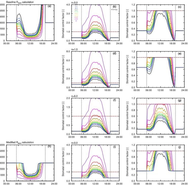
Figure 2 shows the diel cycle of stomatal resistances cal-culated in FORCAsT for each model level within the crown space; an average canopy resistance is also indicated.Rstom
is set to 3000 overnight and falls to a minimum during the middle of the day when light levels are highest in the canopy. Rstom is lower at the top of the canopy and increases with
Stomatal control factor [-]
Stomatal control factor [-]
Stomatal control factor [-]
Stomatal control factor [-]
Stomatal control factor [-]
Stomatal control factor [-]
Stomatal control factor [-]
Stomatal control factor [-]
Figure 2.Stomatal control applied to storage emissions. The top row shows the baseline(a)stomatal resistance,(b)stomatal control factor Rfctas calculated in Eq. (10), and(c)the stomatal control factor as calculated in Eq. (11a) and (b), i.e. with a limiting value of 1.0. Coloured lines show the resistances and control factors as a leaf-area-weighted average for each crown space model level across the 10 leaf angle classes. The crosses show the canopy average weighted by foliage fraction in each level. The second and third rows show the effect onRfct of altering the scaling factor,n, in Eq. (10) (dandf) and Eq. (11a) and (b) (eandg). The bottom row shows the same as the top for the modified stomatal resistance calculations in which “daylight” is assumed to start only when PAR exceeds a threshold of 10.0 µmol m−2s−1.
(Eq. 10) describes the inverse ofRstom, reaching a peak at
midday and having a greater value higher in the canopy. As shown in the middle panels Rfct reaches > 1.0 during the
middle of the day for all but the very lowest canopy lay-ers. Modelled stomatal control (S-simulations) therefore en-hances emissions of methanol and acetaldehyde above those simulated by traditional emissions algorithms during this
models were derived to fit observed emission rates (see e.g. Guenther et al., 1993) and could be assumed to account for this effect.
Hence, a second set of “modified” stomatal control (R-) experiments were performed in which it was assumed that beyond a threshold stomatal aperture, stomatal conductance no longer controls emissions, which continue unhindered once the stomates are considered to be fully open. Beyond this point, emissions from storage pools are regulated by temperature alone according to the relationship in Eq. (2), i.e.Rfctin Eq. (9) takes a value of unity, thus assuming that
traditional emissions algorithms correctly capture emission rates during the middle of the day. Within FORCAsT this was modelled using a threshold function:
Rfct= 3000
n·Rstom, Rfct<1.0 (11a)
Rfct=1.0, at all other times. (11b) The use of the function shown in Eqs. (11a) and (b) limits the temporal extent of stomatal control on methanol and ac-etaldehyde emissions for most canopy layers to the transi-tion times of day (dawn and dusk) when the stomata are ei-ther opening or closing as light levels increase or decrease. This is consistent with results from controlled experiments and observations by Niinemets and Reichstein (2003a) that indicate that stomatal aperture has only a transient effect on the emissions of oVOCs and is negligible under steady-state light conditions. It should be noted however that under the average July radiation conditions, the lower canopy levels do not receive sufficient PAR to reach this threshold value within FORCAsT.
3 Results
3.1 Summary of observations
July was roughly the middle of the growing season in 2012 with emissions unaffected by springtime leaf flush or autumn senescence. As observed previously at many sites, fluxes of both methanol and acetaldehyde are highly variable, with pe-riods of net positive and net negative exchange (e.g. McKin-ney et al., 2011; Wohlfahrt et al., 2015; Karl et al., 2005). In prior years, concentrations of methanol at Harvard For-est remained high even outside of the spring emissions peak (McKinney et al., 2011).
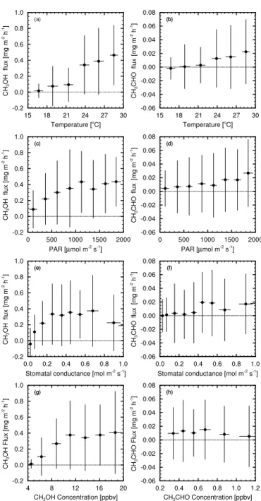
Figure 3 shows correlations of the observed daytime (05:00–19:00 EST) fluxes of methanol and acetaldehyde dur-ing July 2012 with air temperature, PAR, canopy stomatal conductance, and concentrations of methanol and acetalde-hyde. Canopy stomatal conductance for the tower footprint was estimated from energy fluxes measured at Harvard For-est following the methodology of Shuttleworth et al. (1984) to calculate surface resistances. The raw data were highly
flux flux
flux
flux
flux
flux
Figure 3.Observed daytime (05:00–19:00 EST) fluxes of methanol (left) for July 2012 vs.(a)air temperature, (c)PAR, (e)canopy stomatal conductance, and(g) methanol concentration (all mea-sured at 29 m). The right hand column (b, d, f, h) shows the same relationships for acetaldehyde. Temperatures were binned in 2.5◦C intervals, PAR in 250 µmol m−2s−1, stomatal conductance
scattered, and were therefore binned by the independent vari-able in each case, with Fig. 3 showing only the mean values (with bars showing±1 standard deviation to give an
indica-tion of the variability of the data) for each of these bins for clarity. The weak relationships with each of the environmen-tal variables evident in Fig. 3 illustrate the difficulty in iden-tifying the key processes driving canopy-scale exchanges of oVOCs under varying environmental conditions from obser-vations alone.
Canopy-top fluxes of methanol appear to be positively correlated with temperature (Fig. 3a) and to a lesser ex-tent with PAR (Fig. 3c). The correlation with temperature seems to be exponential as might be expected. The contribu-tion of stomatal conductance to observed methanol fluxes is more difficult to interpret, although the data appear to show a strong linear correlation at low conductance, suggesting that at small stomatal aperture the stomata exert control over fluxes of methanol to the extent that it is observable at the canopy scale. However, it is possible that this correlation in-stead reflects correlated responses of emissions and stomatal aperture to increasing light and temperature. The positive re-lationship between canopy-top methanol fluxes and concen-trations at low concentration is likely due to the influence of increasing light and temperature, increasing production of methanol at a greater rate than the loss processes (dry de-position to surfaces within the canopy and chemical loss). At higher concentrations, methanol loss rates increase suffi-ciently to balance production.
Fluxes of acetaldehyde are lower and more variable than those of methanol, and averages are clustered near zero. However, the fluxes do appear to be positively correlated with temperature (Fig. 3b), although the relationship is weaker and does not appear to be exponential. There is no dis-cernible correlation between acetaldehyde fluxes and either PAR (Fig. 3d) or stomatal conductance (Fig. 3f). This might suggest that acetaldehyde emissions are not controlled by stomatal aperture but may rather indicate the influence of the greater number of sources and sinks for acetaldehyde at the spatial and temporal scale of the canopy. Jardine et al. (2008) describe a clear negative correlation between acetaldehyde fluxes and concentrations measured in the laboratory. Fig. 3h could be interpreted in a similar way, although the correlation here (at the canopy scale) is far weaker.
The weakness of the observed correlations and the vari-ability of the observed fluxes are a reflection of the com-plexity of in-canopy processes and interactions, all of which (emissions, photochemical production and loss, and turbu-lent exchange) are strongly influenced by temperature, while only photolysis and direct foliage emissions are directly de-pendent on light levels (although the penetration of radiation into the canopy drives both leaf temperature and turbulence).
3.2 Baseline
When FORCAsT is driven in default mode with average me-teorology and initial conditions for July 2012 and primary emissions of only isoprene and monoterpenes, the model fails to capture either the magnitude or diurnal profile of the observed concentrations and fluxes of methanol and acetalde-hyde at 29 m (Fig. 4a–d, black lines). For both methanol and acetaldehyde, FORCAsT simulates negative fluxes at all times, with a pronounced decrease during daylight hours (Fig. 4a and c). In contrast, fluxes measured by eddy co-variance show strongly positive (upward) exchange occur-ring duoccur-ring the day and fluxes near zero at night. Observed concentrations increase to 12.8 (methanol) and 0.72 ppbv (acetaldehyde) during daylight hours, dipping sharply after dusk and decreasing steadily to a minimum around dawn (Fig. 4b and d). By contrast the baseline modelled concen-trations of both compounds decrease throughout the 24 h pe-riod, (Fig. 4b and d), suggesting strong daytime sources of both methanol and acetaldehyde within the canopy, which FORCAsT does not simulate with the default model settings. 3.3 Biogenic emissions of methanol and acetaldehyde
(E-simulations)
Leaf-level measurements of methanol emissions have demonstrated that all C3vegetation types emit methanol at
rates on par with the major terpenoids (Fall and Benson, 1996). Given the lack of other in situ sources of methanol, the diel cycle of fluxes and concentrations that is gener-ally absent from anthropogenic and transported sources, and the magnitude of the underestimation of canopy-top fluxes (ranging from ∼0.01 overnight to 0.7 mg m−2h−1 in the
early afternoon), it seems likely that there are substantial foliage emissions of methanol at Harvard Forest (see also McKinney et al., 2011). Furthermore, the diurnal profile, strongly reminiscent of isoprene, suggests that the emissions are both light and temperature dependent.
While the magnitude of the missing acetaldehyde fluxes is lower (between∼0.01 and 0.05 mg m−2h−1), the diel
cy-cles of both fluxes and concentrations is similar to those of methanol. This again suggests relatively strong leaf-level emissions of acetaldehyde at this site. It is likely that the absolute concentrations and fluxes are lower since primary emissions of acetaldehyde have generally been found to be a factor of 2–10 lower than those of methanol (Seco et al., 2007; Karl et al., 2003; Guenther et al., 2012).
Figure 4.Measured (grey circles with vertical bars indicating 1 standard deviation above and below the mean) and modelled (solid lines) fluxes (left) and concentrations (right) at 29 m for an average day in July 2012 for methanol(a)fluxes (mg m−2h−1)and(b)concentrations
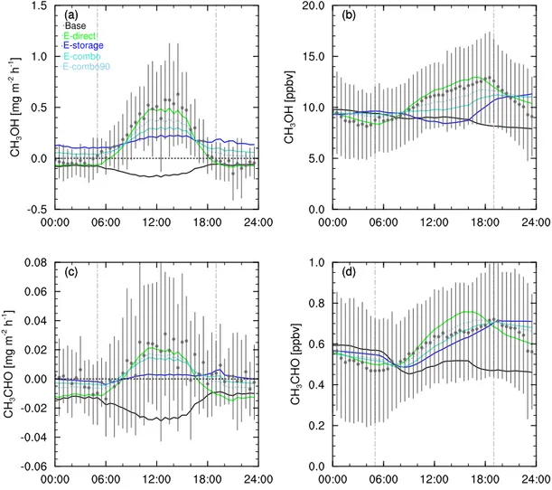
(ppbv) and acetaldehyde(c)fluxes and(d)concentrations. The solid black line shows the baseline model simulation. Coloured lines denoteE -direct (green),E-storage (blue), andE-combo (cyan) simulations in which direct, storage, and combination emissions pathways respectively are included. The dashed turquoise line shows theE-combo90 (combo emissions with 90 direct and 10 % storage emission pathways) sensitivity test. Dashed grey vertical lines show dawn and dusk. Times shown are Eastern Standard Time (EST).
the most densely foliated level where emissions also peak. This feature is less evident in the case of acetaldehyde (Fig. 5g), demonstrating its greater number of sources and sinks. Chemical production and loss is highest at the top of the canopy and the boundary layer just above due to the higher levels of radiation and temperature driving OH radical formation and reaction rates. For both oVOCs, it is emissions and deposition, both leaf-level processes governed by the stomata, that dominate production and loss; chemistry con-tributions are at least an order of magnitude lower. However, both chemistry and turbulent transport contribute to the com-plexity evident in the evolution of concentrations and fluxes and the high degree of variability seen in the observations (see e.g. Figs. 3 and 5).
Difficulties in simultaneously reconciling both fluxes and concentrations of methanol and acetaldehyde are also likely a result of the complexity of in-canopy processes. Figure 5
shows that the top of the canopy is a region of abrupt transi-tion for the sources and sinks of oVOCs with emissions and deposition limited to the canopy and a sudden change in tur-bulent mixing above the foliage. The heterogeneity of con-centrations, concentration gradients, and fluxes of methanol and acetaldehyde in time and space are evident from Fig. 5, demonstrating that the level at which model and measure-ments are compared can also affect the measured–modelled bias.
3.3.1 Methanol
-1
-1
-1
-1
(g) (h) (i)
(j) (k) (l)
Figure 5.Production and loss within the canopy space for methanol:(a)concentration,(b)chemical production rate (including photolysis),
Figure 6.As Fig. 4 with blue lines showingE-storage, orange linesS-storage simulations, and turquoise and yellow lines showingE-combo andS-combo simulations respectively. The dashed turquoise line shows theE-combo90 sensitivity test. Panels show(a)methanol fluxes,
(b)methanol concentrations,(c)acetaldehyde fluxes, and(d)acetaldehyde concentrations at 29 m.
modelled fluxes of methanol are positive when storage emis-sions are included and peak during the middle of the day, modelled midday fluxes are only around a third of measured fluxes (Fig. 6a, E-storage) and modelled night-time fluxes are well above (∼0.15–0.20 mg m−2h−1) those observed,
which are close to but slightly below zero. The diurnal profile ofE-storage-modelled concentrations is the inverse of mea-sured methanol mixing ratios: elevated at night and decreas-ing toward the middle of the day (Fig. 6b,E-storage). This gives further credence to the light dependence of methanol emissions, which has been identified in numerous other for-est ecosystems (see e.g. Wohlfahrt et al., 2015; Seco et al., 2015; McKinney et al., 2011).
Direct emissions are intrinsically linked to photosynthesis and are therefore strongly dependent on light as well as tem-perature. Introducing purely direct emissions of methanol in FORCAsT (E-direct) reproduces the observed diurnal pro-file of both fluxes and concentrations and succeeds in captur-ing the pronounced daytime peak and sharp drop-off at night
seen in both. Modelled mixing ratios, however, peak slightly in advance of the observed maximum (Fig. 6b,E-direct) and do not drop sharply enough after dusk. Modelled fluxes re-main negative at night (Fig. 4a,E-direct) but are slightly be-low those observed during the dawn transition period, sug-gesting that while methanol emissions are light dependent they may not be purely direct emissions (which drop to zero at night). However, the limitations of eddy covariance flux measurement techniques at night may introduce error into the observation–model comparison.
Combo emissions comprising 80 direct and 20 % stor-age emissions (E-combo) do not reproduce the observed de-crease in fluxes and concentrations at night. Modelled night-time fluxes remain positive and ∼0.05–0.1 mg m−2h−1
a maximum discrepancy of∼1.5–2 ppbv or 15 %) nor drop
as steeply as observations after dusk (Fig. 4b,E-combo). In-creasing the proportion of direct emissions to 90 % (Fig. 4a and b) improves the fit of both fluxes and concentrations at all times with maximum daytime differences reduced to 0.2 mg m−2h−1(∼30 %) and 1.0 ppbv (∼8 %) respectively.
Modelled concentrations still fail to capture the pronounced changes observed at dawn, although this may be the result of boundary layer dilution and canopy flushing.
The E-direct simulation gives the best overall model-measurement fit of the emissions sensitivity tests, emphasis-ing the strong light dependence of methanol emissions pre-viously noted. Including direct emissions in FORCAsT sim-ulates the bidirectional fluxes and a diel cycle of concentra-tions similar to those observed at this site. Such emissions do not fully capture all of the features of the field data, indicat-ing that while methanol emissions are strongly light depen-dent, traditional models of primary biogenic emissions (e.g. MEGAN; Guenther et al., 2012) may not fully account for the fundamental processes driving methanol exchange be-tween the canopy and atmosphere even when a small con-tribution from storage pools (e.g. E-combo90) is included. However, it should be noted that the fluxes especially rep-resent instantaneous assessments of a situation that rapidly fluctuates in both time and space, which may in part account for the discrepancies between model and measurements. 3.3.2 Acetaldehyde
Similar to methanol, introducing storage-only emissions of acetaldehyde does not capture the peak in fluxes during the day (Fig. 4c,E-storage), suggesting that acetaldehyde emis-sions are also light dependent. Modelled concentrations are close to those observed during daylight hours in both mag-nitude and profile, with a maximum difference of∼0.2 ppbv (15 %), but they do not reproduce the observed drop in con-centration just after dusk nor the rapid increase after dawn (Fig. 4d,E-storage). However, the greater complexity of ac-etaldehyde production and loss on the timescales involved in canopy–atmosphere exchange makes interpretation of the concentrations more difficult.
Introducing purely direct emissions of acetaldehyde (E -direct) has the same effect as for methanol. Fluxes are strongly negative at night in FORCAsT (around 0.01– 0.015 mg m−2h−1below observed fluxes; Fig. 4c,E-direct)
and concentrations rise too quickly during the day, peak-ing around 4 h earlier and∼0.10 ppbv (∼15 %) higher than
measured mixing ratios (Fig. 4d,E-direct) with a maximum overestimation of ∼0.15 ppbv (∼25 %). The steep night-time drop in observed fluxes and concentrations is reflected (although overestimated) in the model, but overall the simu-lations suggest acetaldehyde emissions are not purely direct. In contrast to methanol, acetaldehyde fluxes are better rep-resented by the inclusion of combo emissions comprising 80 % direct emissions (Fig. 4c,E-combo). This captures the
diurnal profile of the observations, although not the mid-day peak, and does not exhibit the same variability in fluxes around dawn and dusk (which may be attributable to the previously described limitations of eddy covariance at these times). Modelled concentrations are within∼0.01 ppbv of those observed during daylight hours and drop quickly af-ter dusk (Fig. 4d,E-combo). When the proportion of direct emissions is increased to 90 %, concentrations peak in the late afternoon when measured mixing ratios decline (Fig. 4d, E-combo90). The maximum discrepancy is around half that ofE-direct, and the night-time decrease in mixing ratios is well captured. Daytime fluxes are similar to those of the E-combo simulation but decrease more sharply in the af-ternoon and are lower overnight (∼0.05 mg m−2h−1below
observations). None of the simulations capture the observed dip in concentration in the late afternoon. However, the re-sults suggest that the canopy–atmosphere exchange of ac-etaldehyde may be best represented using the combination of emissions of traditional emissions models, with a “light-dependent” fraction of 80 % as currently suggested (Guen-ther et al., 2012).
3.4 Effect of stomatal conductance on modelled emissions (S-simulations)
We now test the effects of stomatal control on the storage-based emissions mechanism by including stomatal regulation in the storage and combo emissions algorithms. These simu-lations effectively introduce a degree of light dependence to releases of VOCs from storage pools, although it should be noted that the dependence on PAR introduced in this way is not as strong as for direct emissions. We first present and dis-cuss the results of incorporating stomatal control throughout the day (i.e. theS-simulations usingRfctas shown in Eq. 10)
for both methanol and acetaldehyde. The effects of modify-ing the control factor (i.e. the R-simulations using Rfct as
shown in Eq. 11a and b) are described in Sect. 3.5.
3.4.1 Methanol
The inclusion of stomatal control of methanol emissions from storage structures into FORCAsT improves the fit of modelled-to-observed fluxes of methanol for both simula-tions that include storage-type emissions, i.e.S-storage vs. E-storage andS-combo vs. E-combo (Fig. 6a). For 100 % storage emissions (S-storage), daytime fluxes are enhanced, and they exhibit the pronounced midday peak of the measure-ments (generally < 0.2 mg m−2h−1 below those observed).
Night-time fluxes are reduced by ∼0.1–0.15 mg m−2h−1,
indicating a dependence on light that is not adequately repre-sented by including stomatal control.
Modelled fluxes and concentrations for combo emissions (20 % storage emissions) with stomatal control (Fig. 6a,S -combo) mirror those for S-storage, although fluxes remain slightly higher during the middle of the day and drop a lit-tle closer to zero at night, and concentrations continue to rise until around 16:00 EST. However, the diurnal profile of methanol concentrations simulated byE-combo90 emissions without stomatal control is closer to the observed than either of the simulations incorporating stomatal control, and 100 % direct emissions still provides the best overall fit.
3.4.2 Acetaldehyde
The effects of including stomatal control of emissions of acetaldehyde from storage pools (Fig. 6c and d) are simi-lar to those described above for methanol. For 100 % stor-age (S-storage vs.E-storage) emissions the diurnal profile of modelled acetaldehyde fluxes is a good fit to observa-tions (Fig. 6c), with a pronounced peak during the middle of the day (∼0.005–0.01 mg m−2h−1 (maximum 0.03) below
measured fluxes) and dropping below zero overnight (again
∼ 0.005–0.01 mg m−2h−1below measurements). Modelled
concentrations increase too rapidly during the day, peaking
∼0.15 ppbv (∼25 %) above those observed and∼4 h earlier, but they do capture the night-time decrease in concentrations seen in the observations (Fig. 6d).
Model output for theS-combo simulation is almost iden-tical to that for S-storage described above, with the two di-verging only at night when the combo emissions are lower, reducing fluxes and, to a lesser extent, concentrations of ac-etaldehyde. Although introducing stomatal control of emis-sions from storage pools improves the magnitude and diurnal profile of modelled fluxes, acetaldehyde exchanges at Har-vard Forest do not show a strong dependence on stomatal conductance at the canopy scale. Instead they are better rep-resented by the use of traditional emissions models, with a proportion of emissions from storage pools and the remain-der via direct release (with the best fit given by 80 direct and 20 % storage, i.e.E-combo). This is in agreement with the theoretical conclusions reached by Niinemets and Re-ichstein (2003b) and the experimental and field results from Kesselmeier (2001) and Kesselmeier et al. (1997). Jardine et al. (2008) report strong evidence of stomatal control at the leaf and branch level and present field measurements that ap-pear to demonstrate that stomatal regulation is relevant at the ecosystem scale for forests in the USA. While our results do not support this conclusion, the authors did report large differences in the effect of stomatal aperture between tree species (Jardine et al., 2008), which may help explain the ap-parent contradiction.
3.5 Threshold stomatal control (R-simulations)
In theR-simulations, the stomatal control function was mod-ified to limit stomatal regulation of storage emissions to tran-sition periods as outlined in Sect. 2.3.3. This is consistent with laboratory-based observations of transient emissions bursts associated with light–dark transitions, assuming in ef-fect that there is a point at which the stomatal aperture is suf-ficient to no longer be a limiting factor. After this point, we set the stomatal control factor to unity to ensure that emis-sions are no longer dependent on stomatal aperture. This re-stricts differences between emissions, and therefore fluxes and concentrations, modelled in the R- and E-simulations to periods around dawn and dusk.
3.5.1 Methanol
For both R-storage and R-combo simulations, methanol fluxes now show a dip just after dawn and again in the late afternoon, reflecting the period of time when the stomata are partially open (Fig. 7a) but do not otherwise diverge from E-storage or E-combo. Concentrations still match neither the magnitude nor diurnal profile exhibited by the measure-ments, decreasing during the day but taking longer to recover in the late afternoon (Fig. 7b). The effect is more pronounced for 100 % storage emissions, but methanol fluxes and con-centrations measured above the canopy at Harvard Forest are still most closely matched with theE-direct emissions path-way (Fig. 7a, b).
3.5.2 Acetaldehyde
By contrast, acetaldehyde fluxes for theR-storage simula-tion show very little change fromE-storage until late morn-ing (Fig. 7c), whenR-storage fluxes are nearly double those modelled inE-storage but remain well below those observed. Following a steep decline in fluxes in the afternoon to a min-imum just before dusk, the post-dusk spike in fluxes previ-ously noted in the 100 % storage emissions simulations is enhanced. Acetaldehyde concentrations forR-storage differ little fromE-storage during the day but remain elevated at night (Fig. 7d). Introducing stomatal regulation to combo emissions (Fig. 7c, d;R-combo vs.E-combo) has little ef-fect on either fluxes or concentrations. Observed acetalde-hyde fluxes and concentrations are still best reflected byE -combo traditional emissions algorithms without explicit pa-rameterisation of stomatal regulation.
3.6 Scaling factor,n
Figure 7.Simulations of modified stomatal control of storage emissions (R-). Blue and turquoise lines showE-storage andE-combo as in Fig. 6. Red (R-storage) and dashed, dark red (R-storageN6) lines show the effects on 100 % storage emissions for scaling factorn=3 and n=6 respectively. Gold (R-combo) and dashed brown (R-comboN6) lines show the same for combo emissions (20 % storage). Panels show
(a)methanol fluxes,(b)methanol concentrations,(c)acetaldehyde fluxes, and(d)acetaldehyde concentrations at 29 m for an average day in July 2012.
emissions by stomata occurs over too brief of a period to be of significance at an ecosystem scale for highly volatile VOCs. However, Niinemets and Reichstein (2003a, b) pos-tulate that emission rates of highly water-soluble VOCs such as methanol are subject to stomatal regulation over longer timescales, potentially modifying emissions over scales rel-evant to canopy–atmosphere exchange. Niinemets and Re-ichstein (2003b) concluded that the strength and persis-tence of stomatal control on leaf-level emissions scaled with the Henry’s law coefficient. Hence, in the final stom-atal control simulations (R-storageN15, R-storageN6, R -comboN15, andR-combo6) we scaled the “degree” of reg-ulation by altering the scaling factor,n, in Eq. (11a) and (b) (see Table 5), altering both the magnitude and duration of stomatal control (i.e. the time taken for Rfct in Eq. (10) to
reach values over 1.0) as shown in Fig. 2.
Changing n makes little difference to modelled fluxes or concentrations of methanol or acetaldehyde (Fig. 7; R-storageN6 vs. R-storage and R-comboN6 vs. R -combo). Night-time fluxes were enhanced slightly (∼0.02 mg m−2h−1 for 100 % storage emissions and ∼0.01 mg m−2h−1 for 80 % storage emissions) when n was doubled. Concentrations of both were reduced in the late afternoon, reflecting the extended duration of control of emission but the effect is short-lived and is not reflected in the observations. Changes at all times were negligible when nwas reduced to 1.5 (not shown).
the top 20 % of the canopy at Harvard Forest; Parker, 1998), and emission rates are small.
4 Conclusions
When light-dependent emissions of methanol and acetalde-hyde were included, the FORCAsT canopy–atmosphere change model successfully simulated the bidirectional ex-change of methanol and acetaldehyde at Harvard Forest, a northern mid-latitude mixed deciduous woodland. Over-all, we find that the bidirectional exchange of methanol at Harvard Forest is well captured with the algorithms cur-rently used for modelling foliage emissions of oVOCs (e.g. MEGAN; Guenther et al., 2012) assuming 100 % light-dependent (direct) emissions. In the case of acetaldehyde, modelled concentrations prove robust, with a relatively good fit to observations for all emissions scenarios employed here, likely due to the greater number of chemical sources and sinks of acetaldehyde in comparison to methanol. However, we find that canopy-top acetaldehyde fluxes at this site are also best modelled with traditional emissions algorithms. In contrast to methanol, however, acetaldehyde emissions at Harvard Forest appear to be derived from both direct syn-thesis and storage pools, with 80 % direct emissions giving the best overall fit.
The light dependence of both methanol and acetaldehyde emissions at the leaf level has been ascribed to the stomatal control of diffusion from storage pools, which would oth-erwise be expected to be dependent on temperature alone. We incorporated a simple parameterisation of the regulation of emissions according to stomatal aperture into FORCAsT to determine how stomatal control affects canopy-top fluxes and concentrations of methanol and acetaldehyde at this site. While we found that some simulations that included stomatal regulation of emissions showed a good fit to measured fluxes, none proved effective in reproducing both the observed con-centrations and fluxes.
Instead, our simulations show that current emissions algo-rithms are capable of capturing fluxes and concentrations of both methanol and acetaldehyde near the top of the canopy and are therefore appropriate for use at the ecosystem scale. Our results further demonstrate that canopy-top fluxes of methanol and acetaldehyde are determined primarily by the relative strengths of foliage emissions and dry deposition, in-dicating that 3-D atmospheric chemistry and transport mod-els must include a treatment of deposition that is not only dy-namically intrinsically linked to land surface processes but is consistent with the emissions scheme.
Our results show that it is possible to model canopy-top fluxes of methanol and acetaldehyde, and to capture bidirec-tional exchange without the need to include direct represen-tations of stomatal control of emissions. This contrast to ex-perimental evidence highlights the complexity of competing in-canopy processes, which act to buffer the stomatal control
of emissions observed at the leaf and branch level. Stomatal aperture affects emissions over too short of a timescale to be observable at the canopy scale when other sources and sinks are fully accounted for. The times around dawn and dusk, when stomatal regulation has been demonstrated to oc-cur, are also associated with rapid changes in chemistry and atmospheric dynamics, which likely outweigh the small dif-ferences in emission rates. Our findings indicate that the in-clusion of a light-dependent fraction in current emissions al-gorithms (e.g. Guenther et al., 2012) captures the changes in storage emissions due to changes in stomatal aperture suffi-ciently well to simulate exchanges at the canopy scale.
Given that observed methanol fluxes appear strongly cor-related with stomatal conductance at small stomatal aper-tures, it is perhaps surprising that we found no evidence supporting the suggestion that stomatal control of methanol emissions is observable at the canopy scale. We ascribe this to the use of empirically derived emissions algorithms com-bined with the similar and competing strong dependence of methanol deposition on stomatal conductance.
Our results highlight the importance of the holistic treat-ment and coupling between land surface sources and sinks. The use of explicit and consistent dynamic representations of emissions and deposition, which dominate the in-canopy budgets for these longer-lived oVOCs, are needed in atmo-spheric chemistry and transport models. Such an approach would adequately account for the role of the stomata in both processes and allow bidirectional exchange to be success-fully simulated without the need for including either leaf-level process detail or a compensation point.
However, this study also demonstrates the need for a bet-ter understanding and representation of the complex rela-tionship between turbulence, fluxes, and concentration gradi-ents within and above the forest canopy. Such understanding can only be achieved through further modelling studies at a range of scales in combination with robust measurements of concentrations and fluxes of VOCs, their primary oxidants, and oxidation products at multiple heights within the forest canopy.
5 Data availability
HF066 (http://harvardforest.fas.harvard.edu:8080/exist/ apps/datasets/showData.html?id=hf066), and HF069 (http://harvardforest.fas.harvard.edu:8080/exist/apps/ datasets/showData.html?id=hf069). Flux and concentra-tion data from the 2012 intensive field campaign will be transferred to the Harvard Forest data archive for long-term storage and access in the future.
Acknowledgements. This material is based upon work supported by the National Science Foundation under Grant No. AGS 1242203. The Harvard Forest Flux Tower is an AmeriFlux core site funded in part by the US Department of Energy’s Office of Science and additionally by the National Science Foundation as part of the Harvard Forest Long Term Ecological Research site.
Edited by: L. Ganzeveld
Reviewed by: two anonymous referees
References
Ashworth, K., Chung, S. H., Griffin, R. J., Chen, J., Forkel, R., Bryan, A. M., and Steiner, A. L.: FORest Canopy Atmo-sphere Transfer (FORCAsT) 1.0: a 1-D model of bioAtmo-sphere- biosphere-atmosphere chemical exchange, Geosci. Model Dev., 8, 3765– 3784, doi:10.5194/gmd-8-3765-2015, 2015.
Baldocchi, D.: A multi-layer model for estimating sulfur dioxide deposition to a deciduous oak forest canopy, Atmos. Environ., 22, 869–884, doi:10.1016/0004-6981(88)90264-8, 1988. Baldocchi, D. D.: Assessing the eddy covariance technique
for evaluating carbon dioxide exchange rates of ecosystems: past, present and future, Glob. Change Biol., 9, 479–492, doi:10.1046/j.1365-2486.2003.00629.x, 2003.
Baldocchi, D.: Measuring fluxes of trace gases and energy between ecosystems and the atmosphere – the state and future of the eddy covariance method, Glob. Change Biol., 20, 3600–3609, doi:10.1111/gcb.12649, 2014.
Baldocchi, D. D., Hicks, B. B., and Camara, P.: A canopy stomatal resistance model for gaseous deposition to vegetated surfaces, Atmos. Environ., 21, 91–101, 1987.
Barford, C. C., Wofsy, S. C., Goulden, M. L., Munger, J. W., Pyle, E. H., Urbanski, S. P., Hutyra, L., Saleska, S. R., Fitzjarrald, D., and Moore, K.: Factors Controlling Long- and Short-Term Sequestra-tion of Atmospheric CO2in a Mid-latitude Forest, Science, 294, 1688–1691, doi:10.1126/science.1062962, 2001.
Blackadar, A. K.: High-resolution models of the planetary boundary layer, in: Advances in Environmental Science and Engineering, Gordon and Breech Science Publishers, Inc., NewYork, USA, 1, 50–85, 1979.
Bryan, A. M., Bertman, S. B., Carroll, M. A., Dusanter, S., Edwards, G. D., Forkel, R., Griffith, S., Guenther, A. B., H ansen, R. F., Helmig, D., Jobson, B. T., Keutsch, F. N., Lefer, B. L., Press-ley, S. N., Shepson, P. B., Stevens, P. S., and Steiner, A. L.: In-canopy gas-phase chemistry during CABINEX 2009: sensitivity of a 1-D canopy model to vertical mixing and isoprene chemistry, Atmos. Chem. Phys., 12, 8829–8849, doi:10.5194/acp-12-8829-2012, 2012.
Bryan, A. M., Cheng, S. J., Ashworth, K., Guenther, A. B., Hardiman, B. S., Bohrer, G., and Steiner, A. L.: Forest-atmosphere BVOC exchange in diverse and structurally com-plex canopies: 1-D modeling of a mid-successional for-est in northern Michigan, Atmos. Environ., 120, 217–226, doi:10.1016/j.atmosenv.2015.08.094, 2015.
Butler, T. M., Taraborrelli, D., Brühl, C., Fischer, H., Harder, H., Martinez, M., Williams, J., Lawrence, M. G., and Lelieveld, J.: Improved simulation of isoprene oxidation chemistry with the ECHAM5/MESSy chemistry-climate model: lessons from the GABRIEL airborne field campaign, Atmos. Chem. Phys., 8, 4529–4546, doi:10.5194/acp-8-4529-2008, 2008.
Chen, J. and Griffin, R. J.: Modeling Secondary Organic Aerosol Formation From Oxidation of α-Pinene, β -Pinene, and d-Limonene, Atmos. Environ., 39, 7731–7744, doi:10.1016/j.atmosenv.2005.05.049, 2005.
Environmental Protection Agency (EPA): National and Regional Air Quality Trends, vailable at: https://gispub.epa.gov/air/ trendsreport/2016/ (last access: 10 December 2016), 2015. Fall, R. and Benson, A.: Leaf Methanol – the Simplest
Nat-ural Product From Plants, Trends Plant Sci., 1, 296–301, doi:10.1016/S1360-1385(96)88175-0, 1996.
Fischer, E. V., Jacob, D. J., Yantosca, R. M., Sulprizio, M. P., Mil-let, D. B., Mao, J., Paulot, F., Singh, H. B., Roiger, A., Ries, L., Talbot, R. W., Dzepina, K., and Pandey Deolal, S.: Atmospheric peroxyacetyl nitrate (PAN): a global budget and source attribu-tion, Atmos. Chem. Phys., 14, 2679–2698, doi:10.5194/acp-14-2679-2014, 2014.
Forkel, R., Klemm, O., Graus, M., Rappenglück, B., Stockwell, W. R., Grabmer, W., Held, A., Hansel, A., and Steinbrecher, R.: Trace gas exchange and gas phase chemistry in a Norway spruce forest: A study with a coupled 1-dimensional canopy at-mospheric chemistry emission model, Atmos. Environ., 40, 28– 42, doi:10.1016/j.atmosenv.2005.11.070, 2006.
Folberth, G. A., Hauglustaine, D. A., Lathière, J., and Brocheton, F.: Interactive chemistry in the Laboratoire de Météorologie Dy-namique general circulation model: model description and im-pact analysis of biogenic hydrocarbons on tropospheric chem-istry, Atmos. Chem. Phys., 6, 2273–2319, doi:10.5194/acp-6-2273-2006, 2006.
Ganzeveld, L., Eerdekens, G., Feig, G., Fischer, H., Harder, H., Königstedt, R., Kubistin, D., Martinez, M., Meixner, F. X., Scheeren, H. A., Sinha, V., Taraborrelli, D., Williams, J., Vilà-Guerau de Arellano, J., and Lelieveld, J.: Surface and boundary layer exchanges of volatile organic compounds, nitrogen oxides and ozone during the GABRIEL campaign, Atmos. Chem. Phys., 8, 6223–6243, doi:10.5194/acp-8-6223-2008, 2008.
Gao, W., Wesely, M. L., and Doskey, P. V.: Numerical Modeling of the Turbulent Diffusion and Chemistry of NOx, O3, Isoprene,
and Other Reactive Trace Gases in and Above a Forest Canopy, J. Geophys. Res., 98, 18339–18353, 1993.
Geron, C., Rasmussen, R., Arnts, R. R., and Guenther, A.: A Review and Synthesis of Monoterpene Speciation From Forests in the United States, Atmos. Environ., 34, 1761–1781, 2000.
Goel, N. S. and Strebel, D. E.: Simple beta distribution represen-tation of leaf orienrepresen-tation in vegerepresen-tation canopies, Agron. J., 76, 800–802, 1984.