Profiles of CH4, HDO, H2O, and N2O with improved lower tropospheric vertical resolution from Aura TES radiances

(1)

AMTD

4, 6679–6721, 2011

Profiles of CH₄, HDO, H₂O, and N₂O

J. Worden et al.

Title Page Abstract Introduction Conclusions References Tables Figures

◭ ◮

Back Close Full Screen / Esc

Printer-friendly Version Interactive Discussion

Discussion

P

a

per

|

Dis

cussion

P

a

per

|

Discussion

P

a

per

|

Discussio

n

P

a

per

|

Atmos. Meas. Tech. Discuss., 4, 6679–6721, 2011 www.atmos-meas-tech-discuss.net/4/6679/2011/ doi:10.5194/amtd-4-6679-2011

Atmospheric Measurement Techniques Discussions

This discussion paper is/has been under review for the journal Atmospheric Measurement Techniques (AMT). Please refer to the corresponding final paper in AMT if available.

Profiles of CH

₄

, HDO, H

₂

O, and N

₂

O with

improved lower tropospheric vertical

resolution from Aura TES radiances

J. Worden1, S. Kulawik1, C. Frankenberg1, V. Payne2, K. Bowman1, K. Cady-Peirara2, K. Wecht3, J.-E. Lee1, and D. Noone4

1

Jet Propulsion Laboratory/California Institute of Technology, Pasadena, CA, USA

2

Atmospheric and Environmental Research, Lexington, MA, USA

3

Earth and Planetary Sciences, Harvard University, MA, USA

4

Department of Atmospheric and Oceanic Sciences, and Cooperative Institute for Research in Environmental Sciences, University of Colorado, Boulder, CO, USA

Received: 21 August 2011 – Accepted: 18 October 2011 – Published: 3 November 2011 Correspondence to: J. Worden (john.worden@jpl.nasa.gov)

(2)

AMTD

4, 6679–6721, 2011

J. Worden et al.

◭ ◮

Discussion

P

a

per

|

Dis

cussion

P

a

per

|

Discussion

P

a

per

|

Discussio

n

P

a

per

|

Abstract

Thermal infrared (IR) radiances measured near 8 microns contain information about the vertical distribution of water vapor (H2O), one of its minor isotopologues (HDO) and methane (CH₄), key gases that can be used to investigate the water and carbon cycles. Here, we show improvements in vertical resolution and reduction in uncer-5

tainties for estimates of these trace gases made from the Aura Tropospheric Emission Spectrometer (TES). The improvements are achieved by utilizing more of the inherent information available in the TES measurements. In previous versions of the TES profile retrieval algorithm, a “spectral-window” approach was used that attempted to minimize uncertainty from interfering specie. However, this approach can also reduce the verti-10

cal resolution of the retrieved species. Here we document the vertical sensitivity and error characteristics of retrievals in which H2O, HDO, CH4and nitrous oxide (N2O) are jointly estimated (together with temperature, surface emissivity, and cloud properties) using the spectral region between 1100 cm−1 and 1330 cm−1. The TES retrieval con-straints are also modified to maximize the use of this information. The H2O estimates 15

show greater vertical resolution in the lower troposphere and boundary layer, while the new HDO/H₂O estimates can now profile the HDO/H₂O ratio between 925 hPa and 450 hPa in the tropics and during summertime at high latitudes. The new retrievals are now sensitive to methane in the free troposphere between 800 and 150 mb with peak sensitivity near 650 hPa. However, there is a bias in the upper troposphere of approx-20

imately 10 % that is likely related to temperature uncertainties and/or to errors in the methane spectroscopy. We discuss approaches for correcting this bias either through averaging or through correcting the estimated methane using co-estimated N₂O pro-files. While these new CH4, HDO/H2O, and H2O estimates are consistent with previous TES retrievals in the regions of overlap, future comparisons with independent profile 25

(3)

AMTD

4, 6679–6721, 2011

J. Worden et al.

◭ ◮

Discussion

P

a

per

|

Dis

cussion

P

a

per

|

Discussion

P

a

per

|

Discussio

n

P

a

per

|

1 Introduction

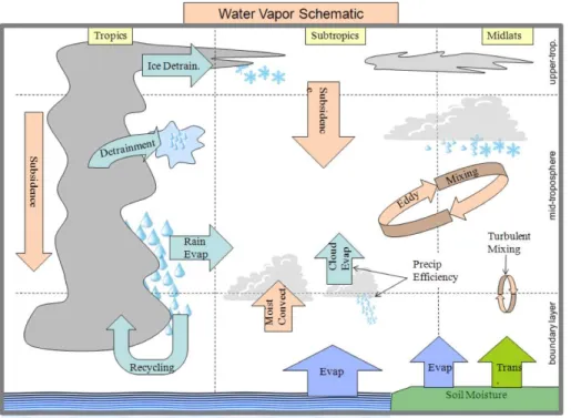
Investigating the processes controlling the water and carbon cycles and their linkages require multiple tracers that are sensitive to the vertically distributed sources, sinks, and processes controlling the water and carbon cycles. For example, Fig. 1a shows a schematic (Brown, 2011) of the vertical distribution of moisture sources, sinks, and 5

exchange processes in the troposphere. Measurements of water vapor profiles (e.g., Dessler et al., 2007, and references therein), upper tropospheric water (e.g., Reed et al., 2008) and the vertical distribution of clouds (e.g., Stephens and Vane, 2007; Su et al., 2008) have been used to examine the exchange and transport processes con-trolling tropospheric humidity. Measurements of the isotopic ratio of water can provide 10

an additional constraint for quantifying the distribution of the sources and exchange processes through the sensitivity of this composition to that of the moisture source, to changes in phase, and to transport and mixing processes (e.g., Kuang et al., 2003; Worden et al., 2006, 2007; Risi et al., 2008; Nassar et al., 2007; Payne et al., 2007; Brown et al., 2008; Noone et al., 2008; Frankenberg et al., 2009; Herbin et al., 2009; 15

Steinwagner et al., 2010). Satellite measurements such as those from TES, the At-mospheric Chemistry Experiment (ACE), the Infrared AtAt-mospheric Sounding Interfer-ometer (IASI), and the SCanning Imaging Absorption SpectroMeter for Atmospheric CHartographY (SCIAMACHY) have been used for this purpose. Similarly, any of the dynamical processes controlling the water cycle such as surface exchange, mixing, 20

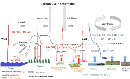
advection, and convection also affect the carbon cycle. Figure 1b shows a schematic of the sources, sinks, and dynamics affecting atmospheric CO₂ and CH₄ methane (adopted from Sarrat et al., 2010). As with water, mixing processes in the free tropo-sphere (e.g., Jiang et al., 2008; Li et al., 2010; Lee et al., 2007; Risi et al., 2008) and boundary layer (e.g., Stephens et al., 2007a; Picket-Heaps et al., 2011; Querino et al., 25

(4)

AMTD

4, 6679–6721, 2011

J. Worden et al.

◭ ◮

Discussion

P

a

per

|

Dis

cussion

P

a

per

|

Discussion

P

a

per

|

Discussio

n

P

a

per

|

Consequently, in order to investigate the processes, sources, and sinks affecting the global carbon and water cycles it is useful to have vertically resolved trace gas profiles. It is with this motivation that we seek to improve the vertical resolution of the TES H2O, HDO, and CH₄products, especially in the lowermost troposphere and boundary layer where many of the exchange processes between the surface, boundary layer, and free 5

troposphere have significant impact on the tropospheric distribution of these gases. In this paper we show that a simultaneous retrieval of H₂O, HDO, CH₄and N₂O us-ing spectral radiances from the TES instrument (Beer et al., 2001) between 1150 and 1340 cm−1 will result in improved vertical resolution and uncertainties for TES geo-physical retrievals over the previous TES results. We first present an overview of the 10

previous (use of spectral micro-windows to minimize interference errors) and new (joint estimate) TES retrieval approaches. We then present an overview of the error char-acteristics and vertical resolution for H2O, HDO/H2O and CH4 profiles. We also show how referencing the estimated methane profile to the jointly retrieved N₂O results can theoretically reduce systematic errors, most notably from temperature, in the methane 15

profile estimate; however, improved a priori distributions of N2O are required before we fully exploit this potential error reduction. Comparisons between the new and old estimates are shown in the altitude regions where the sensitivities overlap for HDO and H2O. Validation of the new retrievals where vertical sensitivity has been increased will be discussed in subsequent papers.

20

2 The TES instrument and trace gas retrieval overview

The TES instrument is an infrared, high spectral resolution, Fourier Transform spec-trometer covering the spectral range between 650 to 3050 cm−1 (15.4 to 3.3 µm) with an apodized spectral resolution of 0.1 cm−1 for the nadir view (Beer et al., 2001). Spectral radiances measured by TES are used to infer atmospheric profiles using a 25

(5)

AMTD

4, 6679–6721, 2011

J. Worden et al.

◭ ◮

Discussion

P

a

per

|

Dis

cussion

P

a

per

|

Discussion

P

a

per

|

Discussio

n

P

a

per

|

2006), subject to the constraint that the parameters are consistent with a statistical a priori description of the atmosphere (Rodgers, 2000; Bowman et al., 2006) . TES pro-vides a global view of tropospheric trace gas profiles including ozone, water vapor and its isotopes, carbon monoxide and methane, along with atmospheric temperature, sur-face temperature, sursur-face emissivity, e_ffective cloud top pressure, and e_ffective cloud 5

optical depth (Worden et al., 2004; Kulawik et al., 2006b; Eldering et al., 2007).

3 Retrieval approach

3.1 Spectral windows

A common approach when performing retrievals from high resolution Fourier transform spectrometers such as TES is to select spectral windows for each target atmospheric 10

constituent that maximize information gained from a spectral measurement and min-imize the systematic errors related to incorrect knowledge of temperature, emissivity, spectral errors, or radiative interference from un-retrieved species (e.g., Echle et al., 2000; Dudhia et al., 2002; Worden et al., 2004; Kuai et al., 2010). The details of the approach for the TES spectral window selection are described in Worden et al. (2004). 15

The general procedure is to first compute an error budget for a set of spectral windows using the following equation:

ˆ

x=x_a+A_xx(x−x_a)+A_xy(y−y_a)MG_zm₊X

i

MG_zKi_b(bi−bi_a) (1)

where ˆx is the estimate of interest and the subscript “a” indicates that a priori knowledge is used for the corresponding vector. TheA_xx is the averaging kernel ma-20

trix describing the sensitivity of the estimate to the true state: A=∂xˆ

∂x. TheAxy is the

(6)

AMTD

4, 6679–6721, 2011

J. Worden et al.

◭ ◮

Discussion

P

a

per

|

Dis

cussion

P

a

per

|

Discussion

P

a

per

|

Discussio

n

P

a

per

|

as discussed in Worden et al., 2004, and Bowman et al., 2006). The vectorm_{is the} measurement noise as a function of wavelength. Thebterm represents un-retrieved parameters that affect the observed radiance withK_bbeing the Jacobian or sensitivity of those terms to the radiance. TheGis the gain matrix, which is the partial derivative of the retrieval parameters to the radiance (F):

5

G_z=∂z

∂F=

KT_zS−_m1K_z+Λz

−1

KT_zS−_m1, (2)

whereS_m is the covariance of the measurement noise for an ensemble of measure-ments andΛz is a constraint matrix used to regularize the retrieval.

The last term in Eq. (1) is the sum over all terms that are not retrieved with the state vector x _{but which also a}_ff_{ect the measured or modeled radiance. Since in general}

10

the noise vector and the errors in these parameters are not exactly known we instead estimate their second order statistics to calculate the errors inx_{from each term:}

Stot=(Axx−I)Sa(Axx−I)T+AxySyATxy+Sm+

X

i

Sb_i (3)

where these four terms correspond to the terms in Eq. (1):Stotis the total error, the next term dependent onS_ais the “smoothing error” which describes how well the estimate 15

can infer the natural variability of the atmosphere (Rodgers, 2000). The third term depending onS_y is similar to the smoothing error and characterizes the impact of the natural variability of jointly estimated parameters on the parameters of interest (Worden et al., 2004). TheSM is the measurement error related to noise, and the summation is

over all un-retrieved parameters (b) which could include spectroscopic uncertainties, 20

temperature, or un-retrieved species.

In general, spectral window selection involves calculating whether a measurement adds information (using a definition of Shannon information content that is related to a decreases uncertainty) using the following equation:

∆H₌1

2log2

_|_S

x1| |S_x2|

=1

2 log2|Sx1| −log2|Sx2|

(7)

AMTD

4, 6679–6721, 2011

J. Worden et al.

◭ ◮

Discussion

P

a

per

|

Dis

cussion

P

a

per

|

Discussion

P

a

per

|

Discussio

n

P

a

per

|

whereH is the information content,S_x₁ is the error covariance before adding a mea-surement andSx2is the error covariance after adding a measurement.

For the previous TES methane retrieval, HDO, H2O, and N2O were treated as ra-diatively interfering species, and similarly CH₄ was considered to interfere with the spectral features of H2O and HDO. For example, if a given spectral point measurement 5

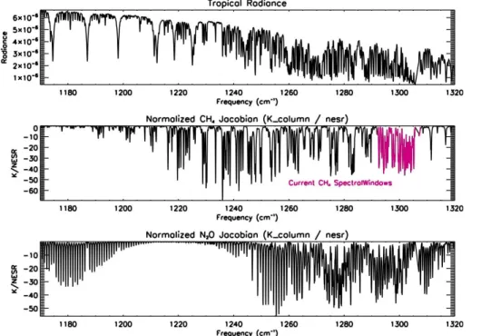
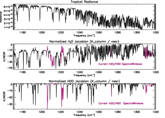
were highly sensitive to methane then it would add uncertainty (as shown in Eq. 1) to the HDO/H2O retrieval. The net information gain (Eq. 4) would likely be negative for the HDO/H₂O estimate and that spectral point would not be used. To illustrate this problem, Fig. 2a and b shows TES measured radiances and calculated Jacobians for CH4, N2O, H2O, and HDO for a tropical ocean scene. The Jacobians have been nor-10

malized by the TES measurement noise and integrated over the whole atmospheric column. The spectral regions colored in red are the spectral regions used for TES v5 retrievals. The CH4 windows were selected to the methane window reduce interfer-ences from H₂O and HDO. N₂O lines are present throughout the CH₄ region and are practically impossible to window around. Similarly, the spectral windows for HDO and 15

H2O were selected to reduce interference from CH4. Figure 2a and b also illustrates high sensitivity to CH₄illustrates that, HDO, H₂O, and N₂O across a wide region. In order to make full use of the spectral information available without negatively adding information content it is necessary to jointly retrieve all constituents together (Worden et al., 2004). If all constituents are jointly retrieved then the last term in Eq. (3) be-20

comes zero and all data points increase the information content. Our approach then is to use effectively the entire spectral range shown in Fig. 2 to jointly estimate HDO, H₂O, N₂O, and methane. However, we currently avoid the a 10 cm−1wide spectral re-gion centered around 1280 cm−1which contains a strong CFC line that is not currently in our atmospheric radiation transfer (forward) model. Other interfering species such 25

(8)

AMTD

4, 6679–6721, 2011

J. Worden et al.

Title Page Abstract Introduction Conclusions References Tables Figures ◭ ◮ ◭ ◮ Back Close Full Screen / Esc

Printer-friendly Version Interactive Discussion Discussion P a per | Dis cussion P a per | Discussion P a per | Discussio n P a per |

3.2 State vector

The new state vector for this joint estimate is:

x₌          

xH₂O

xHDO

xCH₄

xN₂O

Tsurface Pcloud τcloud           =M          

zH₂O

zHDO

zCH₄

zN₂O

Tsurface Pcloud τcloud           (5)

where the vectorsx _{are on a 67 level pressure grid ranging from 1000 hPa to 0.1 hPa} (Worden et al., 2004),Tsurface is the surface temperature,Pcloud is the cloud top pres-5

sure, andτcloud is the cloud effective optical as a function of frequency (e.g., Kulawik et al., 2006b; Eldering et al., 2007). As discussed earlier, the atmospheric species are retrieved on a subset of the 67 level pressure grid used in the TES forward model; this effective hard constraint is described by the mapping matrix “M” and the retrieval levels “z” in Eq. 1) (Worden et al., 2004; Bowman et al., 2006) and must formally be 10

included in the error analysis; however, for the sake of brevity we exclude this term in subsequent equations.

3.3 Constraints

A primary objective for these new TES retrievals is to increase the vertical resolution and information content of methane, H2O, and the HDO/H2O ratio in the lower tropo-15

(9)

AMTD

4, 6679–6721, 2011

J. Worden et al.

◭ ◮

Discussion

P

a

per

|

Dis

cussion

P

a

per

|

Discussion

P

a

per

|

Discussio

n

P

a

per

|

constraints (constraint matrix shown in Eq. 2). Previously, the retrieval levels (z) for H₂O and HDO in the lower troposphere (surface to 500 hPa) tropospheric were de-fined as every other forward model level (x); with the mapping matrix using linear in (log) pressure and (log) mixing ratio to interpolate between retrieval levels and forward model levels. The new retrieval levels in the lower troposphere now have a one-to-5

one mapping with the TES forward model levels for H2O and HDO. For methane, the retrieval level density has been increased from every 3rd level to every 2nd forward model level for CH₄. The constraints were selected based on the altitude-dependent Tikhonov constraints as described in Kulawik et al. (2006a).

In optimal estimation, the constraint matrix is typically calculated from the known 10

a priori statistics of the atmosphere (e.g., Rodgers, 2000). These statistics are most easily generated from global chemical or climate models. However, covariances from these models are not typically invertible, can vary from model to model, and may not replicate actual correlations for molecules such as HDO that are not well observed. We therefore modify the derived correlations from the models by the sensitivity of the 15

radiances to each geophysical parameter (e.g., Kulawik et al., 2006a) or from insight derived from more recent data sets such as water vapor isotope data at the Mauna Loa observatory (Worden et al., 2011). For the new TES retrievals of H2O, HDO, and CH4, the correlation length scales in the constraint matrices (not shown as the larger variance and negative correlations make these plots difficult to generate) have been 20

reduced between the mixing layer (typically surface to 825 hPa) and lower troposphere to reflect conclusions drawn from recent in situ and satellite based observations of these constituents (e.g., Frankenberg et al., 2005, 2009; Worden et al., 2011; Pickett-Heaps et al., 2011; Noone et al., 2011).

4 Comparison of previous (version 6.0 or less) and new profile retrievals

25

(10)

AMTD

4, 6679–6721, 2011

J. Worden et al.

◭ ◮

Discussion

P

a

per

|

Dis

cussion

P

a

per

|

Discussion

P

a

per

|

Discussio

n

P

a

per

|

We also compare old versus new retrievals for the altitude region in which the vertical sensitivities overlap. However, validation of the new data sets in altitude regions where the sensitivity has been improved will be published in subsequent papers.

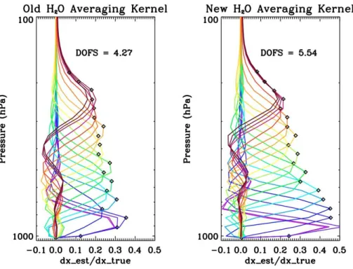
4.1 H₂O

Figure 3a shows the averaging kernels for the new and old H₂O retrievals for a tropical 5

ocean case and Fig. 3b shows the square-root of the diagonals of the corresponding a priori, a posteriori error, and observation covariances. As discussed earlier, the averaging kernels (or rows of the averaging kernel matrix) describe the sensitivity of estimate to the true state, e.g.: A₌∂_∂xxˆ where ˆx is the estimate andx is the true state. As shown in Eq. (1), in the absence of uncertainties, the estimate is related to the true 10

state via the a priori constraint and the averaging kernel matrix (Rodgers, 2000):

ˆ

x=xa+A(x−xa) (6)

An “ideal” averaging kernel would approach the identity matrix. The rows would exhibit narrowly defined peaks, with the peak value of each row located at the pressure of the retrieval level assigned to that row. In the absence of error, the retrieved estimate would 15

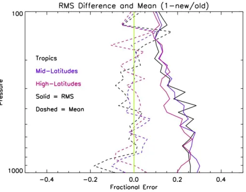
then approach the true state. Figure 3a shows that the H2O averaging kernels have narrower vertical extent and are more distinct for the new retrievals, while Fig. 3b shows that the uncertainties for the new retrieval are overall reduced, except near pressures around 700 hPa for this retrieval.

Figure 4 shows the RMS difference and mean bias between the new (TES Ver-20

(11)

AMTD

4, 6679–6721, 2011

J. Worden et al.

◭ ◮

Discussion

P

a

per

|

Dis

cussion

P

a

per

|

Discussion

P

a

per

|

Discussio

n

P

a

per

|

4.2 HDO/H₂O ratio covariances and mapping

The TES HDO and H2O retrieval approach is designed to reduce the uncertainties in the HDO/H2O ratio estimate as opposed to HDO or H₂O separately (e.g., Worden et al., 2006; Schneider et al., 2006). Consequently, the constraint used to regularize this retrieval is based on an a priori covariance that characterizes the HDO/H2O ratio 5

variability, under the assumption that HDO and H₂O are jointly estimated, i.e.:

Sa=

"

SHa+S

R

a S

H

a

SH_a SH_a

#

(7)

whereSHa is the a priori covariance for H2O andSRa is the a priori covariance for the HDO/H₂O ratio. The a priori covariance for water, S_H, is constructed using statistics from the MOZART (e.g., Brasseur et al., 1998; Horowitz et al., 2003) model but scaled 10

to the expected uncertainty of NCEP water content predictions (Worden et al., 2004). The a priori statistics forS_R are originally based on a version of the National Center for Atmospheric Research (NCAR) Community Atmosphere Model (CAM) (e.g., Collins et al., 2004) that has been modified to predict the isotopic composition of water using the approach developed by Noone and Simmonds (2002). However, we now adjustS_R to 15

reduce correlations between the PBL and the lower troposphere and increase the vari-ance in the boundary layer and free troposphere, consistent with recent observations of the PBL and free troposphere in the subtropics at Mauna Loa (Worden et al., 2010; Noone et al., 2011).

There is no unique averaging kernel for the estimate of the HDO/H2O ratio (Wor-20

den et al., 2006). However, the HDO estimate will always be sensitive to the same air parcels as the H2O estimate. Consequently, the HDO averaging kernel best de-scribes the vertical sensitivity for the HDO/H2O estimate characteristics. The HDO averaging kernel matrix and square root of the diagonal of the HDO/H₂O error covari-ances are shown in Fig. 5 for the same tropical case shown in Fig. 3. The degrees-of-25

(12)

AMTD

4, 6679–6721, 2011

J. Worden et al.

◭ ◮

Discussion

P

a

per

|

Dis

cussion

P

a

per

|

Discussion

P

a

per

|

Discussio

n

P

a

per

|

is a net increase in the error in the boundary layer due to temperature and noise of approximately 3 %. On the other hand, the total error for the HDO/H₂O ratio in the free troposphere has decreased because the increased vertical resolution reduces the smoothing error.

4.2.1 Global comparison of version 6.1 and previous HDO/H2O estimates 5

TES products prior to version 6 have been validated in the lower troposphere by com-paring TES estimates to in situ measurements of HDO and H2O at the Mauna Loa observatory (Worden et al., 2011). While there is insufficient data to provide direct val-idation of the profiles of the new TES HDO/H₂O estimates in the free troposphere, we can compare the new TES estimates in the lower troposphere to the older estimates 10

in the lower troposphere where the sensitivities overlap. This comparison is shown in Fig. 6. The first panel of Fig. 6 shows the latitudinal distribution ofδ−D between the old and new HDO/H2O estimates for the vertical range between 825 and 500 hPa for all scenes in which the degrees of freedom for signal (or trace of the averaging kernel) are larger than 1.0. For a log-based retrieval, the DOF is a good metric for retrieval 15

sensitivity as it indicates how well an ensemble of estimates captures the range of variability of the true distribution. For example, if the DOFS is 0.5 for some altitude range than that means a distribution of estimates, averaged over that altitude, could be expected to capture half the natural variability of the true distribution. The data in the top panel of Fig. 6 are taken from one TES global survey in July 2005. Note that 20

the HDO/H₂O ratio is given in parts per thousand relative to the isotopic composition of ocean water (per mil) orδ−D=1000(R/Rstd−1), where R is the HDO/H2O mole ratio andRstd=3.11×10−

4

is 2 times the isotope ratio of the Vienna Standard mean Ocean water reference for the D/H. As can be seen in this figure, there are many more retrievals at higher latitudes that meet this DOF’s criteria as the sensitivity of the new 25

(13)

AMTD

4, 6679–6721, 2011

J. Worden et al.

◭ ◮

Discussion

P

a

per

|

Dis

cussion

P

a

per

|

Discussion

P

a

per

|

Discussio

n

P

a

per

|

retrieval sensitivity. Figure 6 shows that the RMS difference between the two versions is consistent with the expected uncertainties of the HDO/H2O estimate; however the bias has changed by 7.5 ‰, likely because of the increased number of HDO and H2O lines used for the new estimate.

4.2.2 Global estimates of the HDO/H2O ratio for July 2006 5

A limited number of TES global surveys have been processed with the new retrieval approach and the results are shown in Fig. 7. The top panel of Fig. 7 shows the HDO/H₂O ratio for the altitudes approximately corresponding to the free troposphere (800 to 300 hPa) and the bottom panel shows the HDO/H2O ratio for altitudes that ap-proximately corresponds to the boundary layer (surface to 800 hPa) regions. Values of 10

the HDO/H₂O ratio are given in per mil and have been corrected for the estimated TES bias discussed in the previous section (Worden et al., 2011). Only data in which the DOFS for the HDO estimate is larger than 1 and where the cloud optical depth is less than 0.4 are shown. Note that even though the DOFS can be approximately one, the HDO/H2O profile can still distinguish boundary layer variability from free tropospheric 15

variability of the HDO/H2O ratio as long as the peak values of the averaging kernels (rows of averaging kernel matrix) in these regions are separated; this condition should be met for most clear-sky regions. In the boundary layer above the ocean, mean val-ues of the HDO/H2O ratio are approximately−74 ‰ with an RMS variance of 37 ‰, consistent with the 3 % uncertainty shown for the tropical case in Fig. 5b (for isotopic 20

values near 0.0 a 3 % uncertainty corresponds to 30 ‰ uncertainty). The−74 ‰ mean value for the mean tropical ocean boundary layer is consistent with in situ measure-ments for boundary layer water vapor (e.g., Lawrence et al., 2004; Galewsky et al., 2007; Worden et al., 2011) and therefore suggests that the bias correction calculated for the previous TES HDO/H2O estimates are applicable for these data.

(14)

AMTD

4, 6679–6721, 2011

J. Worden et al.

◭ ◮

Discussion

P

a

per

|

Dis

cussion

P

a

per

|

Discussion

P

a

per

|

Discussio

n

P

a

per

|

4.3 CH₄profiles

In this section we describe the changes in the vertical resolution and error characteris-tics of the new TES CH₄methane retrievals as well as biases in the profiles. We then discuss approaches for correcting or accounting for this bias including averaging, or correcting the methane estimate using the co-retrieved N2O estimate, a temperature 5

based correction is probably also needed. However subsequent analysis using inde-pendent methane data sets will be needed in order to determine the optimal approach for this bias correction.

4.3.1 Vertical sensitivity and resolution

Figure 8a and b shows the averaging kernels for the previous and new CH₄estimate 10

for the same tropical case shown in Figs. 3 and 5 for H2O and HDO. The new CH4 methane profile estimates generally show increased sensitivity to the lower and mid troposphere between 825 and 450 hPa. In addition, the averaging kernels generally peak around 650 hPa and 300 hPa indicating that methane variations at these altitudes can theoretically be distinguished from one another provided the vertical variations 15

are larger than the expected uncertainties. This increased sensitivity to the lower and middle troposphere is due to use of the methane lines around 1230 cm−1 (Fig. 2a) because the lower optical thickness at these wavelengths allows for greater sensitivity to lower tropospheric methane; Fig. 9 shows the DOF’s for the new and older methane retrievals. Typically there are about 0.5 DOFS more for the new retrieval than the old 20

with the increased sensitivity in the middle / lower troposphere.

4.3.2 CH₄error characteristics

(15)

AMTD

4, 6679–6721, 2011

J. Worden et al.

◭ ◮

Discussion

P

a

per

|

Dis

cussion

P

a

per

|

Discussion

P

a

per

|

Discussio

n

P

a

per

|

cross-correlations between adjacent levels (not shown) because methane is a well mixed gas in the free troposphere (e.g., Fung et al., 1991; Wofsy et al., 2011). For this case, the observation error describes the estimated error from noise and from co-retrieved geophysical parameters such as H2O, HDO, surface temperature, and clouds, as well as parameters estimated in a previous step such as O₃ and CO₂. Because 5

temperature is retrieved from a previous step using the CO2ν2 band around 700 cm− 1

, its error estimate is shown separately. As can be seen in this figure, uncertainty due to temperature is the largest component of the methane retrieval error budget in the lower/middle troposphere.

4.3.3 Global distribution of TES observed methane and biases

10

Because of the long life-time of approximately nine years for methane (e.g., Franken-berg et al., 2005) we would expect that methane should be a vertically well mixed gas in the free troposphere (e.g., Wofsy et al., 2011; Pickett-Heaps et al., 2011) but show-ing a latitudinal gradient that depends on inter-hemispheric mixshow-ing, the preponderance of northern hemispheric methane sources relative to the Southern Hemisphere, and 15

the distribution of OH which is the primary sink for CH4(e.g., Fung et al., 1991). Con-sequently, it is reasonable to show a two-dimensional figure of the vertical profile of methane as a function of latitude, averaged over all longitudes as well as ocean and land scenes, in order to infer any vertical biases in the TES methane estimates. Fig-ure 11 shows the TES estimated vertical distribution of methane as a function of lati-20

tude for all data taken during July 2006. A feature of this distribution is that methane is biased high in the upper troposphere and lower stratosphere. This upper tropospheric bias was suspected for previous TES methane estimates that were only sensitive to methane in the upper troposphere (Payne et al., 2009). Based on these observations we suspect that either a systematic bias in temperature is affecting the TES methane 25

(16)

AMTD

4, 6679–6721, 2011

J. Worden et al.

◭ ◮

Discussion

P

a

per

|

Dis

cussion

P

a

per

|

Discussion

P

a

per

|

Discussio

n

P

a

per

|

tropospheric methane estimate as shown in the methane averaging kernels (right panel Fig. 8); in order to determine if this anti-correlation could account for some of this bias we show a global map of the middle troposphere at 618 hPa versus a global map using an information based averaging approach described by Payne et al. (2007) which maps each profile to one or two levels that best represent the altitude where the estimate 5

has the most sensitivity; this approach limits the impact of the a priori on an average because the averaging kernel approaches unity for the re-mapped estimate. For the approach using the Payne et al. (2007) algorithm we only choose methane estimates for which the pressure of the re-mapped (or information averaged) estimate is greater than 450 hPa. Figure 12 (bottom panel) shows global methane estimate from TES for 10

July 2006 for re-mapped estimate. The average pressure for this re-mapped estimate is approximately 500 hPa. Figure 12 (top panel) shows the TES global methane esti-mate for July 2006 for the 562 hPa pressure level. While both maps show an expected latitudinal gradient, the map using the methane estimate from the TES 562 hPa pres-sure level shows un-physically high methane at around −50 degrees relative to the 15

tropics; however, the map derived from the averaged values shows a more realistic latitudinal gradient as compared to previous measurements (e.g., Frankenberg et al., 2006). This result suggests that the anti-correlations in the profile estimate accounts for part of this bias. Future comparisons between the TES data and independent methane measurements will be needed to further characterize this bias so that this data can be 20

used for understanding the global methane cycle. In the next section, we describe an additional approach (e.g., Razavi et al., 2009) in which we correct the methane esti-mate using co-retrieved N₂O estimates. The theoretical calculation of errors using this approach is promising but depends on accurate a priori knowledge of the tropospheric and stratospheric N2O distribution.

25

4.3.4 Methane profile correction using N2O estimate

(17)

AMTD

4, 6679–6721, 2011

J. Worden et al.

◭ ◮

Discussion

P

a

per

|

Dis

cussion

P

a

per

|

Discussion

P

a

per

|

Discussio

n

P

a

per

|

estimates with N₂O shows promise in reducing bias errors, it requires estimates of the a priori distribution of N2O in which the uncertainties in this distribution are much smaller than the uncertainties in CH4. For the current TES estimates, this requirement is not achieved; however, we are looking into obtaining improved a priori distributions of N2O that will meet these requirements.

5

Although N2O varies much less than CH4in the troposphere, the top-of-atmosphere radiance is affected by N₂O and CH₄nearly identically at 8 microns as shown by their normalized column Jacobians in Fig. 2a. We assume here that the tropospheric N2O profile is well represented by the a priori profile, and that deviations in the retrieved N2O from the prior are a result of systematic error. Interference error from temperature, 10

clouds, and emissivity should therefore a_ffect both CH₄ and N₂O very similarly, and correction of CH4 by N2O should therefore reduce the CH4 errors. This correction takes the following form:

ˆ

x_cadj=xˆc−xˆn+xˆan, (8)

wherexc is the estimate for (log) methane,xn is the (log) estimate for N2O, and the 15

adj superscript means “adjusted” or corrected. Because this is simply the ratio of two numbers (for a logarithm) modified by an a priori constraint we can use the same derivation for the errors in the HDO/H₂O estimate as described in Worden et al. (2006) or Schneider et al. (2006). For the methane estimate this leads to:

ˆ

xcadj=xac+(Acc−Anc)(xc−xac)−(Ann−Acn)(xn−xna)+

X

j

(A_cj−A_nj)(xj−xaj) 20

+G_Rm₊_G

R

X

i

Kb_i (b_i−ba_i) (9)

(18)

AMTD

4, 6679–6721, 2011

J. Worden et al.

◭ ◮

Discussion

P

a

per

|

Dis

cussion

P

a

per

|

Discussion

P

a

per

|

Discussio

n

P

a

per

|

affects the jointly retrieved (log) methane estimate (using indices “n” for N₂O and “c” for CH4). The termGr is the gain matrix for the CH4 methane part of the retrieval vector minus that of the N2O part of the retrieval vector (Gr=Gc−Gn). The term GRm is

the impact of measurement noise on the estimate. The index “j” is for jointly retrieved parameters such as H2O or HDO and the index i refers to un-retrieved parameters 5

such as atmospheric temperature, spectroscopy or calibration. Taking the expectation of the adjusted CH₄methane estimate minus the true CH₄methane distribution (e.g., Bowman et al., 2006) yields the second order statistics for Eq. (9):

Sc˜=(Acc−Anc−I)Scc(Acc−Anc−I)

T

+(A_nn−A_cn−I)S_nn(A_nn−A_cn−I)T

+P

j

(Acj−Anj)Sjj(Acj−Anj)

T

+G_RS_mGT_R+G_R(P

i

K_iSi_bKT_i )GT_R (10)

Results show that each term of the cross averaging kernels for the N2O and CH4 es-10

timates are small relative to the averaging kernels for N₂O and CH₄ (A_nc≪A_cc and

Acn≪Ann); consequently we can ignore the cross averaging kernels. Under the as-sumption that the variability of N2O in the atmosphere is much smaller than the vari-ability of CH₄(Wofsy et al., 2011) in the atmosphere we can ignore the term associated withS_nn. This leads to an error estimate for methane, corrected by the N₂O estimate 15

of:

Sc˜=(Acc−I)Scc(Acc−I)T+

X

j

(Acj−Anj)Sjj(Acj−Anj)T+GRSmGTR+GR(

X

i

K_iSi_bKT_i)GT_R

(11)

The right panel of Fig. 10 shows the error budget for these terms. While the observation error (error due to noise and from jointly estimated parameters such as H2O, clouds, 20

(19)

AMTD

4, 6679–6721, 2011

J. Worden et al.

◭ ◮

Discussion

P

a

per

|

Dis

cussion

P

a

per

|

Discussion

P

a

per

|

Discussio

n

P

a

per

|

For example, Fig. 13 shows the two-dimensional (latitude versus altitude) distribution of TES estimated CH₄methane. As compared to Fig. 11, the bias in the upper tropo-sphere is greatly reduced. However, there are now significant “jumps” in the latitudinal variability of the methane distribution that correspond to the discretization of the N2O a priori distribution used for these estimates (Fig. 14). As shown in Eq. (9), there is a 5

term that depends on the difference between the true N2O distribution and the a priori distribution; this term must be effectively zero in order for this correction to be more robust.

5 Summary

This manuscript documents improvements to the Aura TES profile estimates of H2O, 10

HDO/H₂O, and CH₄ by using a joint retrieval over a wide spectral range. In general, the vertical resolution of H2O has increased in the lower troposphere with improved capability to distinguish between boundary layer variability of H2O and that of the free troposphere. Previous (version 5.0 or less) retrievals could not profile the HDO/H₂O ratio but were instead sensitive to an average over the lower troposphere between 550 15

and 825 hPa. New TES estimates of the HDO/H2O profile can now distinguish between the boundary layer/lower troposphere and the middle troposphere around 550 hPa with uncertainties of approximately 30 ‰ for the HDO/H2O ratio in the boundary layer. We show that the new and old estimates for the HDO/H2O estimates are consistent within the expected uncertainties in the regions where the vertical sensitivity overlaps. 20

The new TES methane estimates are now sensitive to methane variability from ap-proximately 800 hPa to 200 hPa whereas previous TES retrievals were only sensitive to methane in the mid- to upper troposphere. However, there is clearly a bias in the upper tropospheric methane that must be better characterized with respect to other parameters that affect the TES methane estimates before this profile information can 25

(20)

AMTD

4, 6679–6721, 2011

J. Worden et al.

◭ ◮

Discussion

P

a

per

|

Dis

cussion

P

a

per

|

Discussion

P

a

per

|

Discussio

n

P

a

per

|

of the sensitivity of the estimate to methane (Payne et al., 2007) We also show both theoretically and empirically that the bias in the estimated methane can be corrected using the co-retrieved N2O estimate; however this correction depends strongly on ex-cellent a priori knowledge of the N2O profile in both the troposphere and stratosphere in which the uncertainty of the a priori distribution is much smaller than the variability 5

of methane. Validation of the new H2O, HDO/H2O, and CH4 profiles in regions with increased vertical sensitivity will require comparisons to independent measurements and will be presented in subsequent papers.

Copyright statement

The author’s copyright for this publication is transferred to California Institute of Tech-10

nology.

Acknowledgements. Government sponsorship is acknowledged.

References

Beer, R., Glavich, T. A., and Rider, D. M.: Tropospheric emission spectrometer for the Earth Observing System’s Aura Satellite, Appl. Optics, 40, 2356–2367, 2001.

15

Bowman, K. W., Rodgers, C. D., Kulawik, S. S., Worden, J., Sarkissian, E., Osterman, G., Steck, T., Lou, M., Eldering, A., Shephard, M., Worden, H., Lampel, M., Clough, S., Brown, P., Rinsland, C., Gunson, M., and Beer, R.: Tropospheric emission spectrometer: Retrieval method and error analysis, IEEE Transactions on Geoscience and Remote Sensing, 44, 1297–1307, 2006.

20

Brasseur, G. P., Hauglustaine, D. A., Walters, S., Rasch, P. J., Muller, J. F., Granier, C., and Tie, X. X.: MOZART, a global chemical transport model for ozone and related chemical tracers 1. Model description, J. Geophys. Res.-Atmos., 103, 28265–28289, 1998.

Brown, D.: Characteristics of Atmospheric Moistening Derived Using Lagrangian Mass Balance From Tropospheric Emission Spectrometer Measurements of HDO and H₂O, PhD Disserta-25

(21)

AMTD

4, 6679–6721, 2011

J. Worden et al.

◭ ◮

Discussion

P

a

per

|

Dis

cussion

P

a

per

|

Discussion

P

a

per

|

Discussio

n

P

a

per

|

Brown, D., Worden, J., and Noone, D.: Comparison of atmospheric hydrology over convective continental regions using water vapor isotope measurements from space, J. Geophys. Res.-Atmos., 113, D15124, doi:10.1029/2007JD009676, 2008.

Clough, S. A., Shephard, M. W., Worden, J., Brown, P. D., Worden, H. M., Luo, M., Rodgers, C. D., Rinsland, C. P., Goldman, A., Brown, L., Kulawik, S. S., Eldering, A., Lampel, M., 5

Osterman, G., Beer, R., Bowman, K., Cady-Pereira, K. E., and Mlawer, E. J.: Forward model and Jacobians for Tropospheric Emission Spectrometer retrievals, Ieee Transactions on Geo-science and Remote Sensing, 44, 1308–1323, 2006.

Dessler, A. E. and Minschwaner, K.: An analysis of the regulation of tropical tropospheric water vapor, J. Geophys. Res.-Atmos., 112, D10120, doi:10.1029/2006JD007683, 2007.

10

Dudhia, A., Jay, V. L., and Rodgers, C. D.: Microwindow selection for high-spectral-resolution sounders, Appl. Optics, 41, 3665–3673, 2002.

Echle, G., von Clarmann, T., Dudhia, A., Flaud, J. M., Funke, B., Glatthor, N., Kerridge, B., Lopez-Puertas, M., Martin-Torres, F. J., and Stiller, G. P.: Optimized spectral microwindows for data analysis of the Michelson Interferometer for Passive Atmospheric Sounding on the 15

environmental satellite, Appl. Optics, 39, 5531–5540, 2000.

Frankenberg, C., Meirink, J. F., van Weele, M., Platt, U., and Wagner, T.: Assessing Methane Emissions from Global Space-Borne Observations, Science, 308, 1010–1014, doi:10.1126/science.1106644, 2005.

Frankenberg, C., Meirink, J. F., Bergamaschi, P., Goede, A. P. H., Heimann, M., Korner, S., 20

Platt, U., van Weele, M., and Wagner, T.: Satellite chartography of atmospheric methane from SCIAMACHY on board ENVISAT: Analysis of the years 2003 and 2004, J. Geophys. Res.-Atmos., 111, D07303, doi:10.1029/2005JD006235, 2006.

Frankenberg, C., Yoshimura, K., Warneke, T., Aben, I., Butz, A., Deutscher, N., Griffith, D., Hase, F., Notholt, J., Schneider, M., Schrijver, H., and Rockmann, T.: Dynamic Processes 25

Governing Lower-Tropospheric HDO/H2O Ratios as Observed from Space and Ground, Sci-ence, 325, 1374–1377, 2009.

Fung, I., John, J., Lerner, J., Matthews, E., Prather, M., Steele, L. P., and Fraser, P. J.: 3-Dimensional Model Synthesis of the Global Methane Cycle, J. Geophys. Res.-Atmos., 96, 13033–13065, 1991.

30

(22)

AMTD

4, 6679–6721, 2011

J. Worden et al.

◭ ◮

Discussion

P

a

per

|

Dis

cussion

P

a

per

|

Discussion

P

a

per

|

Discussio

n

P

a

per

|

Jiang, X., Li, Q. B., Liang, M. C., Shia, R. L., Chahine, M. T., Olsen, E. T., Chen, L. L., and Yung, Y. L.: Simulation of upper tropospheric CO(2) from chemistry and transport models, Global Biogeochem. Cycles, 22, GB4025, doi:10.1029/2007GB003049, 2008.

Kuai, L., Natraj, V., Shia, R. L., Miller, C. and Yung, Y. L.: Channel selection using information content analysis: A case study of CO(2) retrieval from near infrared measurements, Journal 5

of Quantitative Spectroscopy & Radiative Transfer, 111, 1296-1304, 2010.

Kuang, Z. M., Toon, G. C., Wennberg, P. O., and Yung, Y. L.: Measured HDO/H₂O ratios across the tropical tropopause, Geophys. Res. Lett., 30, 1372, doi:10.1029/2003GL017023, 2003. Kulawik, S. S., Osterman, G., Jones, D. B. A., and Bowman, K. W.: Calculation of

altitude-dependent Tikhonov constraints for TES nadir retrievals, Ieee Transactions on Geoscience 10

and Remote Sensing, 44, 1334–1342, 2006a.

Kulawik, S. S., Worden, J., Eldering, A., Bowman, K., Gunson, M., Osterman, G. B., Zhang, L., Clough, S. A., Shephard, M. W., and Beer, R.: Implementation of cloud paper retrievals for Tropospheric Emission Spectrometer (TES) atmospheric retrievals: part 1. Description and characterization of errors on trace gas retrievals, J. Geophys. Res.-Atmos., 111, D24204, 15

doi:10.1029/2005JD006733,2006b.

Lee, J. E., Pierrehumbert, R., Swann, A., and Lintner, B. R.: Sensitivity of stable water iso-topic values to convective parameterization schemes, Geophys. Res. Lett., 36, L23801, doi:10.1029/2009GL040880, 2009.

Li, K. F., Tian, B. J., Waliser, D. E., and Yung, Y. L.: Tropical mid-tropospheric CO(2) variability 20

driven by the Madden-Julian oscillation, Proc. Natl. Acad. Sci. USA, 107, 19171–19175, 2010.

Nassar, R., Bernath, P. F., Boone, C. D., Gettelman, A., McLeod, S. D., and Rinsland, C. P.: Variability in HDO/H2O abundance ratios in the tropical tropopause layer, J. Geophys. Res., 112, D21305, doi:10.1029/2007JD008417, 2007.

25

Nassar, R., Jones, D. B. A., Kulawik, S. S., Worden, J. R., Bowman, K. W., Andres, R. J., Suntharalingam, P., Chen, J. M., Brenninkmeijer, C. A. M., Schuck, T. J., Conway, T. J., and Worthy, D. E.: Inverse modeling of CO₂ sources and sinks using satellite observations of CO₂ from TES and surface flask measurements, Atmos. Chem. Phys., 11, 6029–6047, doi:10.5194/acp-11-6029-2011, 2011.

30

(23)

AMTD

4, 6679–6721, 2011

J. Worden et al.

◭ ◮

Discussion

P

a

per

|

Dis

cussion

P

a

per

|

Discussion

P

a

per

|

Discussio

n

P

a

per

|

a simulation of atmospheric circulation for 1979–1995, J. Climate, 15, 3150–3169, 2002. Noone, D., Galewsky, J., Sharp, Z., Worden, J., Barnes, J., Baer, D., Bailey, A., Brown, D.,

Christensen, L., Crosson, E., Dong, F., Hurley, J., Johnson, L., Strong, M., Toohey, D., Van Pelt, A., and Wright, J.: Properties of air mass mixing and humidity in the subtropics from measurements of the D/H isotope ratio of water vapor at the Mauna Loa Observatory, J. 5

Geophys. Res.-A, in review, 2011.

Payne, V. H., Noone, D., Dudhia, A., Piccolo, C., and Grainger, R. G.: Global satellite mea-surements of HDO and implications for understanding the transport of water vapour into the stratosphere, Q. J. Roy. Meteorol. Soc., 133, 1459–1471, 2007.

Payne, V. H., Clough, S. A., Shephard, M. W., Nassar, R., and Logan, J. A.: Information-10

centered representation of retrievals with limited degrees of freedom for signal: Application to methane from the Tropospheric Emission Spectrometer, J. Geophys. Res., 114, D10307, doi:10.1029/2008JD010155, 2009.

Pickett-Heaps, C. A., Jacob, D. J., Wecht, K. J., Kort, E. A., Wofsy, S. C., Diskin, G. S., Worthy, D. E. J., Kaplan, J. O., Bey, I., and Drevet, J.: Magnitude and seasonality of wetland methane 15

emissions from the Hudson Bay Lowlands (Canada), Atmos. Chem. Phys., 11, 3773–3779, doi:10.5194/acp-11-3773-2011, 2011.

Querino, C. A. S., Smeets, C. J. P. P., Vigano, I., Holzinger, R., Moura, V., Gatti, L. V., Mar-tinewski, A., Manzi, A. O., de Ara ´ujo, A. C., and R ¨ockmann, T.: Methane flux, vertical gradi-ent and mixing ratio measuremgradi-ents in a tropical forest, Atmos. Chem. Phys., 11, 7943–7953, 20

doi:10.5194/acp-11-7943-2011, 2011.

Razavi, A., Clerbaux, C., Wespes, C., Clarisse, L., Hurtmans, D., Payan, S., Camy-Peyret, C., and Coheur, P. F.: Characterization of methane retrievals from the IASI space-borne sounder, Atmos. Chem. Phys., 9, 7889–7899, doi:10.5194/acp-9-7889-2009, 2009.

Read, W. G., Schwartz, M. J., Lambert, A., Su, H., Livesey, N. J., Daffer, W. H., and Boone, 25

C. D.: The roles of convection, extratropical mixing, and in-situ freeze-drying in the Tropi-cal Tropopause Layer, Atmos. Chem. Phys., 8, 6051–6067, doi:10.5194/acp-8-6051-2008, 2008.

Risi, C., Bony, S., and Vimeux, F.: Influence of convective processes on the isotopic composition (delta O-18 and delta D) of precipitation and water vapor in the tropics: 30

2. Physical interpretation of the amount effect, J. Geophys. Res.-Atmos., 113, D19306, doi:10.1029/2008JD009943, 2008.

(24)

AMTD

4, 6679–6721, 2011

J. Worden et al.

◭ ◮

Discussion

P

a

per

|

Dis

cussion

P

a

per

|

Discussion

P

a

per

|

Discussio

n

P

a

per

|

London, World Scientific, 2000.

Sarrat, C., Noilhan, J., Lacarrere, P., Donier, S., Lac, C., Calvet, J. C., Dolman, A. J., Gerbig, C., Neininger, B., Ciais, P., Paris, J. D., Boumard, F., Ramonet, M., and Butet, A.: Atmospheric CO₂ modeling at the regional scale: Application to the CarboEurope Regional Experiment, J. Geophys. Res.-Atmos., 112, D12105, doi:10.1029/2006JD008107, 2007.

5

Schneider, M., Hase, F., and Blumenstock, T.: Ground-based remote sensing of HDO/H₂O ratio profiles: introduction and validation of an innovative retrieval approach, Atmos. Chem. Phys., 6, 4705–4722, doi:10.5194/acp-6-4705-2006, 2006.

Shephard, M. W., Herman, R. L., Fisher, B. M., Cady-Pereira, K. E., Clough, S. A., Payne, V. H., Whiteman, D. N., Comer, J. P., Vomel, H., Miloshevich, L. M., Forno, R., Adam, M., 10

Osterman, G. B., Eldering, A., Worden, J. R., Brown, L. R., Worden, H. M., Kulawik, S. S., Rider, D. M., Goldman, A., Beer, R., Bowman, K. W., Rodgers, C. D., Luo, M., Rinsland, C. P., Lampel, M., and Gunson, M. R.: Comparison of Tropospheric Emission Spectrometer nadir water vapor retrievals with in situ measurements, J. Geophys. Res.-Atmos., 113, D15S24, doi:10.1029/2007JD008822, 2008.

15

Steinwagner, J., Fueglistaler, S., Stiller, G., von Clarmann, T., Kiefer, M., Borsboom, P. P., van Delden, A., and Rockmann, T.: Tropical dehydration processes constrained by the season-ality of stratospheric deuterated water, Nature Geoscience, 3, 262–266, 2010.

Stephens, G. L. and Vane, D. G.: Cloud remote sensing from space in the era of the A-Train, J. Appl. Remote Sens., 1, 013507, doi:10.1117/1.2709703, 2007.

20

Stephens, B. B., Gurney, K. R., Tans, P. P., Sweeney, C., Peters, W., Bruhwiler, L., Ciais, P., Ramonet, M., Bousquet, P., Nakazawa, T., Aoki, S., Machida, T., Inoue, G., Vinnichenko, N., Lloyd, J., Jordan, A., Heimann, M., Shibistova, O., Langenfelds, R. L., Steele, L. P., Francey, R. J., and Denning, A. S.: Weak northern and strong tropical land carbon uptake from vertical profiles of atmospheric CO2, Science, 316, 1732–1735, 2007.

25

Su, H., Jiang, J. H., Gu, Y., Neelin, J. D., Kahn, B. H., Feldman, D., Yung, Y. L., Waters, J. W., Livesey, N. J., Santee, M. L., and Read, W. G.: Variations of tropical upper tropospheric clouds with sea surface temperature and implications for radiative e_ffects, J. Geophys. Res.-Atmos., 113, D10211, doi:10.1029/2007JD009624, 2008.

Wofsy, S. W., S. C., Team, H. S., Team, C. M., and Team, S.: HIAPER Pole-to-Pole Obser-30

(25)

AMTD

4, 6679–6721, 2011

J. Worden et al.

◭ ◮

Discussion

P

a

per

|

Dis

cussion

P

a

per

|

Discussion

P

a

per

|

Discussio

n

P

a

per

|

Worden, J., Kulawik, S. S., Shephard, M. W., Clough, S. A., Worden, H., Bowman, K., and Gold-man, A.: Predicted errors of tropospheric emission spectrometer nadir retrievals from spec-tral window selection, J. Geophys. Res.-Atmos., 109, D09308, doi:10.1029/2004JD004522, 2004.

Worden, J., Bowman, K., Noone, D., Beer, R., Clough, S., Eldering, A., Fisher, B., Goldman, 5

A., Gunson, M., Herman, R., Kulawik, S., Lampel, M., Luo, M., Osterman, G., Rinsland, C., Rodgers, C., Sander, S., Shephard, M., and Worden, H.: Tropospheric Emission Spectrom-eter observations of the tropospheric HDO/H₂O ratio: Estimation approach and characteri-zation, J. Geophys. Res., 111, D16309, doi:10.1029/2005JD006606, 2006.

Worden, J., Noone, D., Bowman, K., and TES science team and data contributors: Importance 10

(26)

AMTD

4, 6679–6721, 2011

J. Worden et al.

◭ ◮

Discussion

P

a

per

|

Dis

cussion

P

a

per

|

Discussion

P

a

per

|

Discussio

n

P

a

per

|

Figure 1a: Sources, sinks, and processes controllin

(courtesy Derek Brown, dissertation)

Fig. 1a. Sources, sinks, and processes controlling tropospheric water vapor (courtesy

(27)

AMTD

4, 6679–6721, 2011

J. Worden et al.

◭ ◮

Discussion

P

a

per

|

Dis

cussion

P

a

per

|

Discussion

P

a

per

|

Discussio

n

P

a

per

|

(courtesy Derek Brown, dissertation)

Figure 1b: sources, sinks, and processes controlling tropospheric

Fig. 1b. Sources, sinks, and processes controlling tropospheric CO₂ and CH₄ (adapted from

(28)

AMTD

4, 6679–6721, 2011

J. Worden et al.

◭ ◮

Discussion

P

a

per

|

Dis

cussion

P

a

per

|

Discussion

P

a

per

|

Discussio

n

P

a

per

|

Fig. 2a. Top: example of radiance measured by TES over a tropical ocean scene. Middle:

(29)

AMTD

4, 6679–6721, 2011

J. Worden et al.

◭ ◮

Discussion

P

a

per

|

Dis

cussion

P

a

per

|

Discussion

P

a

per

|

Discussio

n

P

a

per

|

(30)

AMTD

4, 6679–6721, 2011

J. Worden et al.

◭ ◮

Discussion

P

a

per

|

Dis

cussion

P

a

per

|

Discussion

P

a

per

|

Discussio

n

P

a

per

|

Figure 3a: Averaging kernels for a TES water retrieval using

Fig. 3a. Averaging kernels for a TES water retrieval using old (spectral windows shown in

(31)

AMTD

4, 6679–6721, 2011

J. Worden et al.

◭ ◮

Discussion

P

a

per

|

Dis

cussion

P

a

per

|

Discussion

P

a

per

|

Discussio

n

P

a

per

|

help the reader follow the variability of each averaging kernel with pressure.

(32)

AMTD

4, 6679–6721, 2011

J. Worden et al.

◭ ◮

Discussion

P

a

per

|

Dis

cussion

P

a

per

|

Discussion

P

a

per

|

Discussio

n

P

a

per

|

Fig. 4. The RMS and Mean of the fractional di_fference between the new and old TES H₂O

(33)

AMTD

4, 6679–6721, 2011

J. Worden et al.

◭ ◮

Discussion

P

a

per

|

Dis

cussion

P

a

per

|

Discussion

P

a

per

|

Discussio

n

P

a

per

|

Figure 5a: Averaging kernel for the old and new HDO TES ret

the symbols and colors indicate the pressure level and variat

(34)

AMTD

4, 6679–6721, 2011

J. Worden et al.

◭ ◮

Discussion

P

a

per

|

Dis

cussion

P

a

per

|

Discussion

P

a

per

|

Discussio

n

P

a

per

|

each row of the averaging kernel matrix.

Figure 5b: Same as in Figure 3b but for the HDO/ ratio.

Profiles of CH<sub>4</sub>, HDO, H<sub>2</sub>O, and N<sub>2</sub>O with improved lower tropospheric vertical resolution from Aura TES radiances

AMTD

Profiles of CH

4

, HDO, H

2

O, and N

2

O with

improved lower tropospheric vertical

resolution from Aura TES radiances

AMTD

AMTD

AMTD

AMTD

AMTD

AMTD

AMTD

AMTD

AMTD

AMTD

AMTD

AMTD

AMTD

AMTD

AMTD

AMTD

AMTD

AMTD

AMTD

AMTD

AMTD

AMTD

AMTD

AMTD

AMTD

Figure 1a: Sources, sinks, and processes controllin

(courtesy Derek Brown, dissertation)

AMTD

(courtesy Derek Brown, dissertation)

Figure 1b: sources, sinks, and processes controlling tropospheric

AMTD

AMTD

AMTD

Figure 3a: Averaging kernels for a TES water retrieval using

AMTD

AMTD

AMTD

Figure 5a: Averaging kernel for the old and new HDO TES ret

the symbols and colors indicate the pressure level and variat

AMTD

₄

₂

₂