www.biogeosciences.net/12/5753/2015/ doi:10.5194/bg-12-5753-2015
© Author(s) 2015. CC Attribution 3.0 License.
Annual cycle of volatile organic compound exchange between a
boreal pine forest and the atmosphere
P. Rantala1, J. Aalto2, R. Taipale1, T. M. Ruuskanen1,3, and J. Rinne1,4,5
1Division of Atmospheric Sciences, Department of Physics, University of Helsinki, Helsinki, Finland 2Department of Forest Sciences, University of Helsinki, Helsinki, Finland
3Palmenia Centre for Continuing Education, University of Helsinki, Helsinki, Finland 4Department of Geoscience and Geography, University of Helsinki, Helsinki, Finland 5Finnish Meteorological Institute, Helsinki, Finland
Correspondence to:P. Rantala ([email protected])
Received: 3 June 2015 – Published in Biogeosciences Discuss.: 26 June 2015 Accepted: 25 September 2015 – Published: 9 October 2015
Abstract.Long-term flux measurements of volatile organic compounds (VOC) over boreal forests are rare, although the forests are known to emit considerable amounts of VOCs into the atmosphere. Thus, we measured fluxes of several VOCs and oxygenated VOCs over a Scots-pine-dominated boreal forest semi-continuously between May 2010 and De-cember 2013. The VOC profiles were obtained with a proton transfer reaction mass spectrometry, and the fluxes were cal-culated using vertical concentration profiles and the surface layer profile method connected to the Monin-Obukhov sim-ilarity theory. In total fluxes that differed significantly from zero on a monthly basis were observed for 13 out of 27 mea-sured masses. Monoterpenes had the highest net emission in all seasons and statistically significant positive fluxes were detected from March until October. Other important com-pounds emitted were methanol, ethanol+formic acid, acetone and isoprene+methylbutenol. Oxygenated VOCs showed also deposition fluxes that were statistically different from zero. Isoprene+methylbutenol and monoterpene fluxes fol-lowed well the traditional isoprene algorithm and the hy-brid algorithm, respectively. Emission potentials of monoter-penes were largest in late spring and autumn which was pos-sibly driven by growth processes and decaying of soil lit-ter, respectively. Conversely, largest emission potentials of isoprene+methylbutenol were found in July. Thus, we con-cluded that most of the emissions ofm/z69 at the site con-sisted of isoprene that originated from broadleaved trees.
Methanol had deposition fluxes especially before sunrise. This can be connected to water films on surfaces. Based on this assumption, we were able to build an empirical al-gorithm for bi-directional methanol exchange that described both emission term and deposition term. Methanol emissions were highest in May and June and deposition level increased towards autumn, probably as a result of increasing relative humidity levels leading to predominance of deposition.
1 Introduction
Knowledge on biogenic emissions of volatile organic com-pounds (VOCs) has been continuously increased as a result of a development of modelling methods and extended mea-surement network community (Guenther et al., 1995, 2006, 2012; Sindelarova et al., 2014). VOCs, such as monoterpenes and isoprene, make a major contribution to the atmospheric chemistry, including tropospheric ozone formation, control of atmospheric radical levels, and aerosol particle formation and growth. Therefore, these compounds affect both local and regional air quality and the global climate (Atkinson and Arey, 2003; Kulmala et al., 2004; Spracklen et al., 2008; Kazil et al., 2010).
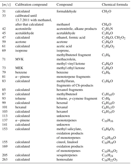
bud-Table 1.The compound names and the formulas listed below in third and fourth column, respectively, are educated estimates for the measured masses (see e.g. de Gouw and Warneke, 2007). However, other compounds also might have a contribution at the measured masses (e.g.
m/z85, see Park et al., 2013). The second column shows whether a sensitivity was determined directly from the calibration or not (derived from a transmission curve, i.e. calculated), and which compounds were used in the calibrations.
[m/z] Calibration compound Compound Chemical formula
31 calculated formaldehyde CH2O
33 calibrated until
13.7.2011 with methanol,
after that calculated methanol CH4O
42 acetonitrile acetonitrile, alkane products C2H3N
45 acetaldehyde acetaldehyde C2H4O
47 calculated ethanol, formic acid C2H6O, CH2O2
59 acetone acetone C3H6O
61 calculated acetic acid C2H4O2
69 isoprene isoprene,
methylbutenol fragment C5H8
71 MVK methacrolein,
methyl vinyl ketone C4H6O
73 MEK methyl ethyl ketone C4H8O
79 benzene benzene C6H6
81 α−pinene monoterpene fragments
83 calculated methylfuran, C5H6O
fragments of C6-products
85 calculated hexanol fragments
87 calculated methylbutenol C5H10O
93 toluene toluene,p-cymene fragment C7H8
99 calculated hexenal C6H10O
101 hexanal hexanal C6H12O
103 calculated hexanol C6H14O
113 calculated unknown
137 α−pinene monoterpenes C10H16
141 calculated unknown
153 calculated methyl salicylate, C8H8O3
oxidation products
of monoterpenes C10H16O
155 calculated cineol, linalool C10H18O
169 calculated oxidation products
of monoterpenes C10H16O2
205 calculated sesquiterpenes C15H24
263 calculated homosalate C16H22O3
get has been estimated to be ca. 10–20 % in carbon basis (Guenther et al., 2012; Sindelarova et al., 2014). Due to their lower reactivity, OVOCs have only a minor role in the bound-ary layer chemistry but they can be transported to the up-per troposphere where, for example, methanol can possibly have a major effect on oxidant formation (Tie et al., 2003; Jacob et al., 2005). Methanol emissions have been widely studied in recent years (e.g. Guenther et al., 2012 and refer-ences therein). However, it has been recently observed that methanol also has significant deposition at some ecosystems. This deposition could be related to the night-time dew on surfaces (Holzinger et al., 2001; Seco et al., 2007; Wohlfahrt et al., 2015) but removal mechanisms of methanol from the surfaces are still unknown (e.g. Laffineur et al., 2012). In
global estimates, methanol deposition is usually determined with a deposition velocity that is tuned to fit concentration observations, leading possibly to uncertainties in methanol budget estimates (Wohlfahrt et al., 2015). Other OVOCs than methanol are even more poorly described in the global scale (Karl et al., 2010).
0 50 100 150 200 250 300 350 2010
2011 2012 2013
Day of year
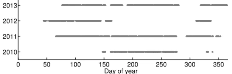
Figure 1.Grey dots show VOC flux data coverage for each year.
In order to describe the VOC exchange processes in mod-els, continuous long-term ecosystem, or canopy, scale flux measurements play an important role (Guenther et al., 2006). They can be used to study the dependencies of these fluxes on environmental variables. Also, even when the process un-derstanding has been obtained by, for example, laboratory experiments, the evaluation of model in ecosystem scale is a crucial step towards reliable global exchange estimates. Un-fortunately, the ecosystem scale flux measurements are rare. As an example, even though branch scale monoterpene emis-sions from Scots pine are well-studied (Ruuskanen et al., 2005; Tarvainen et al., 2005; Hakola et al., 2006; Aalto et al., 2014, 2015), ecosystem scale emissions from Scots pine dominated forests have been mainly explored in short cam-paigns (Rinne et al., 2000b, a, 2007; Ghirardo et al., 2010). Longer time series have also consisted of measurements from May to September only (Räisänen et al., 2009; Taipale et al., 2011). This has had a direct effect on the capability of mod-els to predict monoterpene concentrations (Smolander et al., 2014).
Thus, we have measured ecosystem scale fluxes of VOCs using the proton transfer reaction quadrupole mass spectrom-eter (PTR-MS, Lindinger et al., 1998) above a Scots-pine-dominated forest in Hyytiälä at SMEAR II (Station for Mea-suring Forest Ecosystem–Atmosphere Relations) since 2010. In this study, we quantify the ecosystem scale VOC emis-sions and deposition at a boreal forest site throughout the sea-sonal cycle. The most important ecosystem scale VOCs emit-ted at the site are monoterpenes and methanol (Rinne et al., 2007), thus we concentrate on these compounds separately. Isoprene is also analysed more precisely because despite its importance on a global scale, ecosystem-scale emissions have remained unstudied in Scots-pine-dominated forests.
In the case of monoterpenes and isoprene, we will exam-ine emissions with algorithms suggested by Guenther et al. (1993) and Ghirardo et al. (2010). Our purpose is to study how well the algorithms are able to predict ecosystem-scale fluxes, and how much there is seasonal variation in emis-sion potentials. As the last aim, we examine the importance of the methanol deposition, and develop a simple empirical algorithm describing the bi-directional exchange needed to achieve more precise methanol flux budgets. This algorithm is evaluated against the measurements.
2 Methods and measurements
2.1 Measurement site and VOC concentration calculations
All measurements were conducted in Hyytiälä, Finland, at SMEAR II (Station for Measuring Forest Ecosystem– Atmosphere Relations, 61◦51′N, 24◦17′E, 180 m a.m.s.l., UTC+2). Hyytiälä is located in the boreal region and the dominant tree species in the flux footprint is Scots pine ( Pi-nus sylvestris). In addition to Scots pine, there are some Nor-way spruce (Picea abies) and broadleaved trees such as Eu-ropean aspen (Populus tremula) and birch (Betula sp.). The forest is about 50-years old and the canopy height is currently ca. 18 m. Hari and Kulmala (2005), Haapanala et al. (2007) and Ilvesniemi et al. (2009) have given a detailed description about the station infrastructure and surrounding nature.
The proton transfer reaction quadrupole mass spectrom-eter (PTR-MS, manufactured by Ionicon Analytik GmbH, Innsbruck, Austria) was measuring 27 different masses (see Table 1) using a 2.0 s sampling time from six different mea-surement levels at a tower which was mounted on a pro-truding bedrock, ca. 2 m above the average forest floor. Two of the measurement levels (4.2 and 8.4 m) were below the canopy and four of them (16.8, 33.6, 50.4 and 67.2 m) above it. VOC fluxes were derived from the profile measurements with the surface layer profile method. The temperature was also measured at the VOC sampling levels with ventilated and shielded Pt-100 sensors. A 3-D acoustic anemometer (Gill Instruments Ltd., Solent 1012R2) was installed at the height of 23 m and it was used for determining turbulence parameters, including turbulent exchange coefficients. The photosynthetic photon flux density (PPFD, Sunshine sensor BF3, Delta-T Devices Ltd., Cambridge, UK) was measured at the height of 18 m. The relative humidity (Rotronic AG, MP102H RH sensor) was measured at the height of 16 m.
optimized before a calibration, and we used the same SEM-model (MasCom MC-217) over all years.
The instrumental background was determined every third hour by measuring VOC free air, produced with a zero air generator (Parker ChromGas, model 3501). In addition, the estimated oxygen isotope O17O was subtracted fromm/z33 to avoid contamination of methanol signal. The isotope sig-nal was estimated by multiplying the measured sigsig-nal of
m/z32 by a constant O17O/O2ratio (0.00076, see Taipale et al., 2008). Samples for the zero air generator were taken outside of the measurement cabin close to the ground, and the stability of the zero air generator was followed continuously. We found that the generator had some problems at m/z93
but this did not affect the flux calculations as the same zero air signal was subtracted from each concentration level. 2.2 Flux calculation procedure
The flux of a compound can be written as
F =w′c′= −c
∗u∗, (1)
where c∗= −w′c′/u∗ and u∗= h
(−u′w′)2+(−v′w′)2i1/4 is the friction velocity.
In this study, fluxes were quantified using the surface layer profile method. Detailed description of the flux calculation is given by Rantala et al. (2014), who use the term profile method of this variant of gradient method. Below we give only a brief outline of the method.
According to the Monin-Obukhov theory, a concentration
¯
c(zj)can be calculated at any heightzj in the surface layer using the formula
¯ c(zj)=
c∗
kχ (zj)+ ˙X, (2)
where
χ (zj)≈ln(zM−d)−9h(ζM)− M−1
X
i=j 1
γ (zi, zi+1)
ln
z
i+1−d zi−d
−9h(ζi+1)+9h(ζi)
(3) and
˙
X= ¯c(z0)−c∗ k
ln(z0)−9h(z0/L). (4) Here,k=0.4 is the von Kármán constant (e.g. Kaimal and Finnigan, 1994),9h(ζ )is the integral form of the dimension-less universal stability function for heat,z0is the roughness length, andζ =(z−d)/Lis the dimensionless stability pa-rameter whereLis the Obukhov length (Obukhov, 1971) and
d the zero displacement height.Lhas been derived using di-mensional analysis and it has the following form
L= − u
3 ∗θ¯v
kg(w′θ′ v)s
, (5)
whereθ¯vis the potential virtual temperature,gthe
accelera-tion caused by gravity (g≈9.81 m s−2) and(w′θ′
v)s the tur-bulent heat transfer above the surface (in our case at 23 m).z0 is the surface roughness length,zMthe highest measurement level, and variablesxii+1refer to the average values between heightszi andzi+1. Using the equations above, the surface layer parameter c∗, and the flux, can be derived using the least square estimate (a linear fit).
For the flux calculation procedure, we selectedd=13 m andγ=1.5 between the two lowest levels (Rantala et al., 2014). Between other measurement levels, the roughness sublayer correction factorγwas assumed to be 1, i.e. no
cor-rections were applied. Our lowest and highest measurement levels werez1=16.8 m andzM=67.2 m, respectively. The concentrations,c(zj), were computed as 45 min averages. From 2010 until the end of 2012, the averages from each level consisted of eight data points. From 2013 onwards, two new measurement heights (101 and 125 m) were included in the cycle which reduced the amount of data points (per 45 min) from eight to three at 50.4 m.
Rantala et al. (2014) compared the profile method against the disjunct eddy covariance method. Based on those results, we decided to use the profile method for long-term measure-ments at the site as the DEC-method was often found to have problems in determining low VOC fluxes. For example, the lag-time determination was turned out to be difficult in con-ditions where values are usually close to flux detection limit. Moreover, the high-frequency losses are currently unknown for many VOCs as the response time of the PTR-MS has been studied for water vapour only (Rantala et al., 2014). On the other hand, the profile method has also several systematic error sources because it is an undirect method to measure fluxes, and is based on the parameterization of the surface layer turbulence.
2.3 Flux filtering criteria, a gap-filling and other data processing tools
Periods when the anemometer or the PTR-MS was work-ing improperly, were removed from the time series (Figs. 1 and 2). The fluxes during which ζ <−2, ζ >1 or u∗< 0.2 m s−1 were also rejected from further analysis. Finally,
we disregarded 2.5 % of the lowest and highest values from every month as outliers.
40 60 80 100
RH [%]
2010 2011 2012 2013 average
−10 0 10 20
T [C
°]
0 200 400 600
PPFD [
µ
mol m
−2s −1]
100 150 200 250 300 350 0
50 100
MT flux [ng m
−2
s
−1]
Day of year
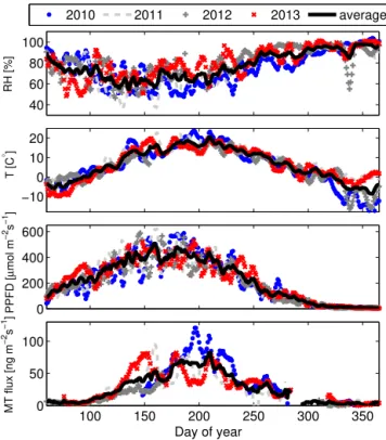
Figure 2. Five-day running averages of relative humidity (RH), temperature (T), PPFD, and gap-filled monoterpene flux (MT flux) for each year as a function of day of year (days 60–365). The thick black solid lines represent averages calculated from the 5-day run-ning means.
In this study, we have often used a relative error,1R, that is defined as
1R=kh−qk
khk , (6)
wherehcorresponds to measured flux values andqto values given by an algorithm. Pearson’s correlation coefficient, r, was used widely through the study as well, and it is hereafter referred as correlation.
Algorithm optimization is applied many times, and all fits were based on, if not stated otherwise, least squares mini-mization and a trust-region-reflective method that is provided as an option in MATLAB (function fit).
2.4 Emission algorithms of isoprene and monoterpenes The well-known algorithm for isoprene emissions (Eiso) is written as
Eiso=Esynth=E0,synthCTCL, (7) whereE0,synth,CT andCLare same as in the traditional iso-prene algorithm (Guenther et al., 1991, 1993). The shape of this algorithm is based on the light response curve of elec-tron transport activity and the temperature dependence of the protein activity. Similar behaviour for methylbutenol (MBO)
emissions from Ponderosa pine has been suggested by for example Gray et al. (2005).
The algorithm we used for monoterpene emissions is the hybrid algorithm
Emt=Esynth+Epool
=E0,hybridfsynthCTCL+(1−fsynth)Ŵ, (8) wherefsynth∈ [0 1]is the ratioE0,synth/E0,hybrid(Ghirardo et al., 2010; Taipale et al., 2011). Epool is the traditional monoterpene algorithm by Guenther et al. (1991) and Guen-ther et al. (1993) and Ŵ=eβ(T−T0) the temperature activ-ity factor, whereβ=0.09 K−1andT
0=303.15 K. The hy-brid algorithm is based on the observation that part of the monoterpene emission even from coniferous trees originates directly from synthesis. Therefore, it can be calculated us-ing an algorithm similar to the isoprene emission algorithm while the rest originates as evaporation from large storage pools (Ghirardo et al., 2010). The latter can be calculated using the exponentially temperature-dependent algorithm, as the temperature dependence of the monoterpene satura-tion vapour pressure is approximately exponential (Guenther et al., 1991, 1993). The formula,
Epool=E0,poolŴ, (9)
is hereafter referred to as the pool algorithm. 2.5 Net exchange algorithm of methanol
The total exchange of methanol consists of both emission term, Emeth, and deposition term,Dmeth. Therefore, an al-gorithm for the methanol flux,Fmeth, has the form of
Fmeth=Emeth−Dmeth. (10)
According to observations, biogenic methanol production is mainly temperature-dependent, with photosynthesis having no direct role (Oikawa et al., 2011). Instead of that, the emissions are potentially controlled by stomatal opening, as methanol has high water solubility, i.e. low Henry’s constant (e.g. Niinemets and Reichstein, 2003; Filella et al., 2009). Therefore, we assumed that part of the emissions could be represented by the traditional temperature activity factorŴ
multiplied by a light-dependent scaling factor of stomatal conductance. In addition, methanol is also produced by non-stomatal sources, such as decaying plant matter (Schade and Custer, 2004; Harley et al., 2007; Seco et al., 2007). More-over, Aalto et al. (2014) observed with chamber studies that at least part of the methanol emissions is independent of light during springtime. Hence, we estimated that the total methanol emission,Emeth, is determined as
Emeth=E0,methfstomataGlight+(1−fstomata)Ŵ, (11)
The light-dependent scaling factor of stomatal conductance,
Glight, was estimated as
Glight≈1−e−α·PPFD, (12)
whereα=0.005 µmol−1m2s is the same as used by Altimir et al. (2004) for pine needles. The stomatal conductance is also dependent on, for example, the temperature and vapour pressure deficit but their effect is much weaker than the effect of light at the site (Altimir et al., 2004). For the temperature activity factor, we used a parameterβ=0.09. In principle,β
should be determined from measurements but we wanted to have as few experimental parameters as possible. Therefore, we used the same value as for monoterpenes.
We assumed that methanol is deposited on wet surfaces, such as on dew, in a way that the methanol concentration at the absorbing surface is zero. Thus, a deposition term,Dmeth, was estimated to be
Dmeth=f (RH)Vd·ρmethanol, (13)
whereρmethanol is a mass mixing ratio measured atz=33.6 m andVda deposition velocity. The functionf (RH)defines a filter of relative humidity (RH) in a such way that
f (RH)= (
0, if RH≤RH0 1, if RH>RH0
(14)
where RH0was determined from the measurements. The de-position velocityVdwas determined by a resistance analogy:
Vd= 1
Ra+Rb+Rw, (15)
where Ra is the aerodynamic resistance, Rb the laminar boundary-layer resistance, andRwa surface resistance. The aerodynamic resistance is written as:
Ra= 1
γ (z1, z2)ku∗
ln
z−d z0
−9h(ζ )
, (16)
where the correction factorγ (z1, z2)=1.5 as with the flux calculations. Rb was determined by a commonly used for-mula (Wesely and Hicks, 1977)
Rb=2(u∗k)−1 κ
η 2/3
, (17)
where η is a diffusivity of methanol and κ a thermal dif-fusivity of air. The factor Rw was assumed to be constant and it was determined from the measurements. In reality,Rw might be also consisting of stomatal uptake due to oxida-tion of methanol into formaldehyde on leaves (Gout et al., 2000). Consequently, the assumption of a constant value is a very rough estimate. However, in order to simplify the al-gorithm as much as possible, the parameterized deposition velocity consisted only of the factorsRa,Rband a constant
Rw. We used the constant values of 1 m and 13×10−6m2s−1 for the surface roughness length (z0) and for the diffusiv-ity of methanol (η), respectively. The diffusivity of methanol was approximated at 273.15 K using Chapman-Enskog the-ory (e.g. Cussler, 1997). Generally, the diffusion coefficient, and thus the deposition velocity, would be larger at higher temperatures. However, using the constant value causes only a minor error. We assumed also a constant value for the ther-mal diffusivity of air (κ=19×10−6 m2s−1).
3 Results and discussion
3.1 Statistical significance of fluxes
For the analysis of seasonal cycle the fluxes were divided into 12 monthly bins, each containing data from a specific month of all years. To study whether the measured fluxes from each month differed significantly from zero or not, numbers of positive and negative fluxes were counted. The null hypoth-esis was that there is no flux, thus the counts of positive and negative values are equal. Finally, it was determined from the binomial distribution with a confidence level of 99.9937 % (“4σ”, Clopper-Pearson method) whether a fraction of pos-itive and negative values could be generated by a random process (the null hypothesis), or if there was a real posi-tive or negaposi-tive flux, i.e. the null hypothesis was rejected. We made the test for both night- (2–8 a.m.) and daytime (11 a.m.–5 p.m.) fluxes separately. Measurements from Jan-uary and FebrJan-uary were excluded from the analysis due to the lack of data points. Measurements at higher mass-to-charge ratio (m/z) than 137 were also left out from the analysis due to a very low sensitivity of the PTR-MS at those masses. In addition, identification of the heavier masses was proven to be extremely difficult.
Altogether, 13 masses (excluding monoterpene fragments atm/z81) had statistically significant fluxes on a monthly scale (Table 2). One should note that the masses for which no significant flux was found (m/z71,m/z79,m/z85,m/z99,
m/z101,m/z103, andm/z113) may have fluxes. This result of the analysis only indicates that with the 4σ criteria, the fluxes of these masses were non-significantly different from zero on a monthly scale.
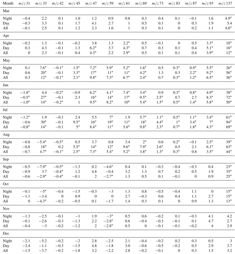
Monoterpenes (m/z137) had the highest net emissions in
every month analysed except in December and November, whereas methanol and acetone (m/z33 andm/z59) showed generally the strongest net deposition. Other important com-pounds emitted or deposited were acetaldehyde (m/z45), ethanol+formic acid (m/z47), acetic acid (m/z61) and iso-prene+methylbutenol (m/z69; Table 2).
Table 2.The table includes daytime, night-time, and diurnal flux averages (arithmetic) for each month (years 2010–2013). The values are expressed with two significant numbers but with a maximum of one decimal. Significant (4σ) averages are marked with an asterisk (∗). A
diurnal average was defined to be statistically significant if either a daytime value or the night-time value differed statistically from zero. The fluxes have unit of ng m−2s−1.
Month m/z31 m/z33 m/z42 m/z45 m/z47 m/z59 m/z61 m/z69 m/z73 m/z83 m/z87 m/z93 m/z137
Mar
Night −0.4 2.2 0.1 1.0 1.2 0.9 0.8 0.3 0.4 0.1 −0.1 1.6 4.9∗
Day −0.3 3.3 0.1 1.7 4.1 2.7 1 0.5 0.1 0 0.3 1.9 5.4
All −0.1 2.5 0.1 1.2 2.3 1.6 1 0.3 0.1 0 0.2 1.1 4.6∗
Apr
Night −0.2 1.3 −0.1 −0.2 3.8 1.3 2.2∗ 0.5 −0.1 0 0.5 3.3∗ 10∗
Day 0.3 4.3 −0.1 1.3 6.2∗ 3.7 4.3∗ 0.7 0.3 0.1 0.4 5.1∗ 16∗
All 0 2.3 −0.1 0.4 4.3∗ 2.2 2.9∗ 0.5 0.1 0.1 0.4 3.9∗ 12∗
May
Night 0.1 7.6∗ −0.1∗ 1.5∗ 7.2∗ 5.9∗ 5.2∗ 1.6∗ 0.5 0.3∗ 0.9∗ 5.5∗ 26∗
Day 0.6 20∗ −0.1 3.3∗ 17∗ 11∗ 11∗ 4.2∗ 1.3 0.3 2.2∗ 9.2∗ 56∗
All 0.3 12∗ −0.1∗ 2.1∗ 9.8∗ 7.3∗ 6.7∗ 2.4∗ 0.7 0.3∗ 1.2∗ 6.5∗ 36∗
Jun
Night −1.8∗ 4.4 −0.2∗ −0.9 6.2∗ 4.1∗ 7.4∗ 3.4∗ 0.9 0.3∗ 0.8∗ 4.9∗ 38∗
Day −0.5∗ 27∗ −0.1 2.3 16∗ 14∗ 17∗ 9.5∗ 2.5∗ 0.7 2.7 8.3∗ 72∗
All −1.0∗ 14∗ −0.2∗ 1 9.5∗ 8.2∗ 10∗ 5.4∗ 1.5∗ 0.5∗ 1.4∗ 5.8∗ 50∗
Jul
Night −1.2∗ 1.9 −0.1 2.4 5.5 7∗ 1.9 5.7∗ 1.1∗ 0.5∗ 1.1∗ 3.4∗ 61∗
Day −0.6 30∗ −0.1 9.5∗ 16∗ 19∗ 11∗ 18∗ 4.4∗ 1∗ 3.4∗ 7∗ 94∗
All −0.8∗ 14∗ −0.1 5∗ 8.4∗ 11∗ 5.6∗ 9.8∗ 2.3∗ 0.7∗ 1.8∗ 4.3∗ 69∗
Aug
Night −0.8 −5.4∗ −0.5∗ 0.5 3.7 0.8 3.4 2∗ 0.6 0.2∗ −0.1 2.5∗ 39∗
Day −0.8 18∗ 0.2 5.5∗ 14∗ 12∗ 9.6∗ 7.9∗ 2.6∗ 0.5 2.1 6.1∗ 63∗
All −0.7 4.7∗ −0.1∗ 2.5∗ 7.3∗ 5.4∗ 5.2∗ 3.8∗ 1.3∗ 0.3∗ 0.8 3.5∗ 44∗
Sep
Night −0.5 −7.9∗ −0.5∗ −1.3 0.2 −4.6∗ 0.4 0.1 −0.3 −0.4 −0.3 0.4 23∗
Day −0.9 3.7 −0.4∗ 1.2 4.8 −0.4 3.2 1.3 0.7 0.2 0.5 1.9 35∗
All −0.6 −2.9∗ −0.4∗ −0.1 2 −2.7∗ 1.3 0.5 0.1 −0.1 0 0.9 25∗
Oct
Night −0.1 −5∗ −0.4 −1.5 −0.3 −3 1.3 0.8 −0.5 −0.4 1.1 0 15∗
Day −1.1 −3.4 0 0.9 0 0 2.7 −0.3 0.6 0.4 1.1 2.7 15∗
All 0 −4.3∗ −0.2 −0.5 0.1 −1.7 1.4 0.3 0.1 0 0.9 1.3 13∗
Nov
Night −1.3 −2.5 −0.1 −1 1.9 −3∗ 0.5 0.6 −0.2 0.1 −0.3 4.1 4.2
Day −0.1 −2.6 −0.3 −1.3 2.2 −2.8∗ 0.6 −0.4 −0.3 −0.1 0.1 4.7 2.7
All −0.4 −3 −0.2 −1.2 2 −2.8∗ 0.5 0 −0.1 −0.1 −0.2 4 2.9
Dec
Night −2.1 −5.2 −0.2 −2 2.8 −2.5 2.1 −0.4 −0.2 0.2 0.3 0.5 3
Day −2.4 −1.1 −0.3 −1.5 4.8 −1.8 3.0 −0.6 −0.5 −0.2 0.5 2.9 3.7
Warneke, 2007). We tried to minimize the interference of water vapour using a normalization method which takes into account changes in water cluster ions (Taipale et al., 2008).
There were also other controversial discoveries such as net emissions ofm/z93. A compound atm/z93 is usually con-nected with toluene but it might be a fragmentation prod-uct ofp-cymene as well (Ciccioli et al., 1999; Heiden et al., 1999; White et al., 2009; Ambrose et al., 2010; Park et al., 2013). We found a dependency between the m/z93 fluxes and E/N whereE is the electric field and N the number density of the gas in the drift tube. This indicates that ob-served positive fluxes could originate at least partly from the monoterpene-relatedp-cymene (Tani et al., 2003).
An interesting result is weak but detectable acetonitrile deposition in June, August and September. Similar obser-vations were done earlier by, for example, Sanhueza et al. (2004) who suggested that acetonitrile is deposited in the tropical savannah ecosystem. Their results imply a deposi-tion velocity of ca. 0.1 cm s−1 for acetonitrile. Our depo-sition velocities were somewhat higher as the typical ace-tonitrile concentration was around 100 ng m−3, and the flux values around−0.5 ng m−2s−1. This corresponds to the de-position velocity of 0.5 cm s−1. According to Dunne et al. (2012), m/z42 signal might be affected by alkanes. The
m/z42 concentration also had a correlation with m/z71 (r=0.57),m/z85 (r=0.47) andm/z99 (r=0.38) concen-trations (typical alkane fragments, see Erickson et al., 2014). Thus, also other compounds than acetonitrile might have a contribution to the measured signal ofm/z42. However, no
correlations were seen between measuredm/z42 and alkane
fluxes. Fluxes of m/z71,m/z85 and m/z99 were actually even statistically insignificant (Table 2). Therefore, we con-cluded that acetonitrile had a major contribution to the ob-served deposition ofm/z42.
The measured fluxes do have significant uncertainties. Some of these are random in nature and will thus cancel out with data analysis of a sufficiently large data set. Some of the uncertainties are more systematic and may bias average flux values presented. The surface layer profile method itself may have a systematic error of about 10 % (Rantala et al., 2014). In addition, monoterpene fluxes are underestimated up to a few percent by the chemical degradation (Spanke et al., 2001; Rinne et al., 2012; Rantala et al., 2014). Our calibration procedure may also contain systematic error sources. This concerns especially the indirect calibration if molecules are fragmented, such as in the case of methylbutenol atm/z87 (Taipale et al., 2008). In addition to systematic errors, ran-dom flux uncertainties are also several hundreds of percent for many compounds (Rantala et al., 2014). On the other hand, when averaging over a sample size of ca. a hundred data points, a random uncertainty of the average is decreased to the scale of 10 %.
After the addition of a mass flow controller to the cali-bration system on 7 July 2011, the sensitivities of methanol were observed to be highly underestimated. The reason was
0 200 400 600 800 1000 1200
0 0.2 0.4 0.6 0.8 1
PPFD [µmol m−2s−1]
Normalized isoprene/MBO flux [ng m
−2
s
−1]
May Jun Jul Aug
CL
A
0 200 400 600 800 1000 1200
0 0.2 0.4 0.6 0.8 1
PPFD [µmol m−2s−1]
Normalized methanol flux
Apr May Jun Jul Aug Sep Glight
B
Figure 3. Temperature normalized isoprene+MBO (a) and methanol(b)fluxes (bin-medians) as a function of PPFD (May–
August and April–September, respectively; years 2010–2013). The isoprene fluxes were normalized by multiplying the measured val-ues by a factor ofCT−1(Eq. 7) whereas the methanol fluxes were multiplied by a factor ofŴ−1(Eq. 11). In addition, values for each month were scaled to the range of[0−1]. Those periods when rela-tive humidity was larger than 75 % were rejected from the methanol analysis to avoid deposition.
unknown but the biased sensitivities were probably caused by an absorption of methanol on metal surfaces of the mass flow controller (Kajos et al., 2015). Therefore, methanol con-centrations were derived from general transmission curves (indirect calibration) after that date (Table 2). The indirect calibration might potentially lead to large systematic errors. However, no rapid changes in the methanol concentrations were observed after 7 July 2011.
3.2 Monoterpene and isoprene fluxes 3.2.1 Isoprene or MBO?
men-tion that typically only 25 % of the ions is detected atm/z87. As the identification of compound observed atm/z69 is not unambiguous, we analysed the fluxes of this mass in more detail to determine if it is more likely to be isoprene or MBO. MBO is produced by conifers (Harley et al., 1998) whereas many broad-leaved trees are high isoprene emitters (Sharkey and Yeh, 2001; Rinne et al., 2009).
In order to quantify the emission potentials for iso-prene+MBO, measured flux values were fitted against the isoprene algorithm (Eq. 7) for each month separately. We found a significant correlation between the measurements and the calculated emissions from May, June, July and Au-gust (Table 3). Here we defined that the measurements and the calculated values correlated significantly if the p value
(p) of the correlation (r) was smaller than 0.0027 (3σ
-criteria). In June, July, and August, the measured fluxes were also clearly light-dependent (Fig. 3). Shapes of the curves in Fig. 3 go near to zero when PPFD is zero and the normalized values have also their saturation point around PPFD=500 µmol m−2s−1 whereC
L is also already larger than 0.8 (Fig. 3). In May, the dependency between the mea-sured fluxes and light was, however, unclear. However, the calculated values corresponded well with the measured ones as is seen in Fig. 4.
Previous emission studies with chamber method with gas chromatography have shown that Scots pines emit MBO much more than isoprene (Tarvainen et al., 2005; Hakola et al., 2006). However, emission potentials of MBO in those studies were only around 2–5 % of emission potentials of to-tal monoterpenes whereas in this study, we found the ecosys-tem scale emission potentials of m/z69 to be around 15– 25 % of emission potentials of monoterpenes. Thus, MBO emissions from Scots pines cannot fully explainm/z69 flux. On the other hand, we may be able to explain the m/z69 emission if we assume that isoprene emission from the mix-ture of spruce, aspen and willow within the footprint area make a considerable contribution in the ecosystem scale emission.
Hakola et al. (2006) observed that maximum MBO emis-sion potential of Scots pine occurs around May and June, and Aalto et al. (2014) showed that the increased MBO emissions during early summer were related to new biomass growth. In the case of isoprene emissions from aspen, the maximum should come later in July (Fuentes et al., 1999). In this study, the maximum emission potential of m/z69
was observed in July, indicating that most of the emissions ofm/z69 might actually consist of isoprene. Maximum net emissions ofm/z87 were also detected in July (Table 2) but the temperature and light normalized fluxes ofm/z87 were largest in May as expected. Even though quantifying the ratio between the MBO and isoprene emissions based on PTR-MS measurements alone is somewhat speculative.
3.2.2 Monoterpenes, their emission potentials and differences to branch scale studies
Monoterpenes are emitted by Scots pine (Hakola et al., 2006), Birch (Hakola et al., 2001) and forest floor (Hellén et al., 2006; Aaltonen et al., 2011, 2013) at the site. Ac-cording to Taipale et al., 2011, Scots pine is the most im-portant monoterpene source in summer but its fraction of the total emission in spring and autumn have remained unstud-ied. Therefore, monoterpene fluxes from spring- and autumn-time will be analysed more carefully in this chapter.
Unsurprisingly, a seasonal cycle of monoterpene fluxes correlated roughly with the temperature (Fig. 2). To exam-ine a response of monoterpene fluxes to the temperature and light in more detail, the fluxes were fitted against the hybrid algorithm and the pool algorithm (Eqs. 8 and 9) for each month separately (Fig. 5). We found a correlation (p value was smaller than 0.0027) between the measurements and the hybrid algorithm from April to October (Table 4).
Significant monoterpene fluxes were also observed in March but no dependence with the temperature was found. This is most probably due to the low temperatures and its diurnal variation, letting the random variation in the flux data to dominate. In addition, Aalto et al. (2015) observed that freezing–thawing cycles may increase the monoterpene emission capacity of Scots pine shoots; in late autumn and early spring such cycles are frequent and potentially hide the relation between temperature and emissions at least partially. Nevertheless, monoterpene fluxes in March were in a reason-able range being lower than in April (Treason-able 2, Fig. 6).
Correlations between measured fluxes and the hybrid emission algorithm were better than those between measured fluxes and the pool algorithm in every month analysed (Ta-ble 4). In addition, relative errors (Eq. 6) between the mea-sured fluxes and the hybrid algorithm were also smaller than the relative errors between the measured fluxes and the pool algorithm. Thus, the hybrid algorithm worked better than the pool algorithm in every month. The result was expected as Taipale et al. (2011) showed that ecosystem scale monoter-pene emission from Scots pine forest, measured by the dis-junct eddy covariance method, has a light-dependent part. In addition, Ghirardo et al. (2010) have shown by stable iso-tope labelling that a major part of the monoterpene emis-sions from conifers originates directly from synthesis (de novo). In this study, the ratiosfsynth=Esynth/Epool varied between 0.36 (July) and 0.79 (October) whereas Ghirardo et al. (2010) estimated that the fraction of the de novo emis-sions from Scots pine seedlings to be around 58 %, and Taipale et al. (2011) estimated the fraction to be around 40% for the Scots pine ecosystem. Generally, these estimates fit well with our results considering the relatively large uncer-tainties (Table 4).
interan-−60 −40 −20 0 20 40 60 80 −60
−40 −20 0 20 40 60 80
Measured methanol flux [ng m−ss−1]
Calculated methanol flux [ng m
−ss
−1
]
1:1
Apr May Jun Jul Aug Sep
10 20 30 40 50
10 20 30 40 50
Measured isoprene+MBO flux [ng m−ss−1]
Calculated isoprene+MBO flux [ng m
−ss
−1
]
1:1
May Jun Jul Aug
50 100 150 200 250 50
100 150 200 250
Measured MT flux [ng m−ss−1]
Calculated MT (hybrid) flux [ng m
−ss
−1
]
1:1
Apr May Jun Jul Aug Sep Oct
50 100 150 200 250 50
100 150 200 250
Measured MT flux [ng m−ss−1]
Calculated (pool) MT flux [ng m
−s
s
−1
]
1:1
Apr May Jun Jul Aug Sep
Figure 4.Calculated values versus measured methanol, isoprene and monoterpene fluxes for each month. Measured monoterpene fluxes have been compared against both hybrid and pool algorithm.
Table 3.The table presents isoprene+MBO emission potential of a synthesis algorithm,E0,synth, including 95 % confidence intervals (years 2010–2013). The table shows also correlations coefficients (r), relative errors between the measurements and the calculated values (1R), and a ratio,Fa/F, whereFais an average value given by the algorithm andF an average value of the measurements. If thepvalue of a correlation was larger than 0.0027, the result was disregarded as statistically insignificant, and those values are not shown in the table.
Month E0,synth r Fa/F 1R
[ng m−2s−1] [%]
May 36±5 0.42 (n=503,p <10−4) 1.09 81 Jun 52±4 0.67 (n=361,p <10−4) 1.02 59 Jul 63±4 0.77 (n=397,p <10−4) 0.98 49 Aug 40±4 0.61 (n=402,p=1.7×10⁻⁴) 1.05 68
nual variation of the potentials was considerably large in May. The emission potentials of May varied from 210 (2012) to 470 ng m−2s−1 (2013) whereas in July, the range was from 200 (2013) to 290 ng m−2s−1 (2010). The high vari-ability might be connected to the differences in the temper-atures as the average tempertemper-atures were 12 and 8.5◦C in May 2013 and in May 2012, respectively. Overall, the high springtime monoterpene emissions have been connected to new biomass growth, including the expansion of new cells, tissues and organs (Aalto et al., 2014), photosynthetic spring
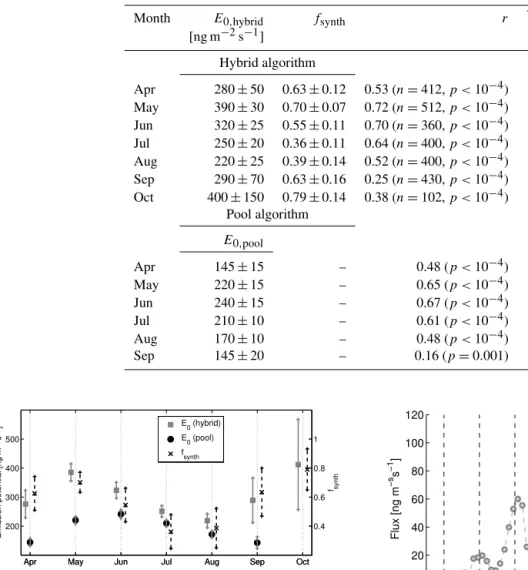
Table 4.The table presents monoterpene emission parameters of a hybrid algorithm,E0,hybrid, andf, including 95 % confidence intervals (years 2010–2013). The table shows also correlations coefficients (r), relative errors between the measurements and the calculated values (1R), and a ratio,Fa/F, whereFa is an average value of the calculated emissions, andF an average value of the measurements. There are also corresponding values of the pool algorithm. If thepvalue of a correlation was larger than 0.0027, the result was disregarded as statistically insignificant, and those values are not shown in the table.
Month E0,hybrid fsynth r Fa/F 1R
[ng m−2s−1] [%]
Hybrid algorithm
Apr 280±50 0.63±0.12 0.53 (n=412,p <10−4) 0.98 64 May 390±30 0.70±0.07 0.72 (n=512,p <10−4) 0.98 48 Jun 320±25 0.55±0.11 0.70 (n=360,p <10−4) 0.99 48 Jul 250±20 0.36±0.11 0.64 (n=400,p <10−4) 0.99 46 Aug 220±25 0.39±0.14 0.52 (n=400,p <10−4) 0.98 55 Sep 290±70 0.63±0.16 0.25 (n=430,p <10−4) 0.94 81 Oct 400±150 0.79±0.14 0.38 (n=102,p <10−4) 0.96 69
Pool algorithm
E0,pool
Apr 145±15 – 0.48 (p <10−4) 1.05 66
May 220±15 – 0.65 (p <10−4) 1.07 54
Jun 240±15 – 0.67 (p <10−4) 1.06 51
Jul 210±10 – 0.61 (p <10−4) 1.02 48
Aug 170±10 – 0.48 (p <10−4) 1.01 56
Sep 145±20 – 0.16 (p=0.001) 0.98 83
Apr May Jun Jul Aug Sep Oct
200 300 400 500
Emission potential [ng m
−2s
−1
]
Apr May Jun Jul Aug Sep Oct
0.4 0.6 0.8 1
fsynth E
0 (hybrid)
E0 (pool) fsynth
Figure 5. Monoterpene emission potentials of both hybrid algo-rithm and pool algoalgo-rithm, andfsynthfor each month (years 2010– 2013). Plus signs show 95 % confidence intervals (Table 4).
the direct comparison of the emission potentials between the seasons difficult.
The hybrid algorithm matched with measurements espe-cially well from May until July when 1R <50 % andr >
0.6. Conversely to those months, the measurements from Oc-tober were noisy leading to somewhat unreliable fitting pa-rameters (Table 4 and Fig. 5). Compared to earlier estimates on autumn monoterpene emissions based on extrapolation of short measurement campaigns (e.g. Rinne et al., 2000a), the autumnal monoterpene emissions were larger than expected. Although one should keep in mind that the data set of this study from October was relatively small, and the results are therefore less representative than from other months.
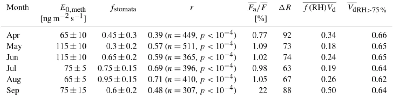
Never-Mar Apr May Jun Jul Aug Sep Oct Nov 0
20 40 60 80 100 120
Flux [ng m
−s s −1 ]
Figure 6.Diurnal cycles (hourly medians) of monoterpene fluxes from March until November (years 2010–2013). The measurements were performed at 0200, 0500, 0800, 1100, 1400, 1700, 2000, and 2300 UTC+2, and the dashed lines represent the noon time.
40 60 80 100 0
20 40 60 80 100 120
RH
Flux [ng m
−2
s
−1
]
Figure 7. Temperature and PPFD classified (12◦C≤T ≤15◦C
and PPFD≤50 µmol m−2s−1) monoterpene fluxes (grey circles, bin-medians,n=15) from May-Aug (years 2010–2013) as a func-tion of relative humidity (RH). Thick black lines represent 95 % confidence intervals of the medians, and grey dots are the measured fluxes.
In addition to the temperature and light intensity, monoter-pene emissions have been also connected to other abiotic stresses, such as mechanical damage, high relative humidity, drought, and increased ozone level (e.g. Loreto and Schnit-zler, 2009 and references therein). At the ecosystem level, such stress-related emissions could often increase monoter-pene fluxes. Thus, they will be incorporated into emission potentials even though the pool algorithm or the hybrid al-gorithm cannot describe those stress emissions at a process level. We found, for example, a weak dependency between relative humidity and monoterpene fluxes in low (PPFD<
50 µmol m−2s−1) light conditions (Fig. 7). Nevertheless, the measured mean fluxes differed from the predicted mean emissions only a few percent on a monthly basis, i.e. in our data set clear signals of stress-related emissions in a temporal scale of 1 month were not found (see also Fig. 4).
Overall, there were some results that were not totally cor-responding with previous monoterpene studies. According to Hakola et al. (2006), monoterpene emissions from two Scots pine branches were highest in June with the (pool) emission potential of ca. 200 ng m−2s−1 (calculated using a needle biomass density of 540 g m−2) whereas the corresponding ecosystem scale emission potential was 240 ng m−2s−1 in our study. The numbers are quite close to each other. How-ever, the difference could also mean that ca. 85 % of monoter-pene emissions would be originated from Scots pines in June and 15 % from other sources, such as a ground vege-tation. The result is realistic as the monoterpene concentra-tions close to the ground and canopy top are almost equal,
02:00 08:00 14:00 20:00 1
2 3 4 5 6
HH:MM
Height index VMR [ppb
v
]
2 2.1 2.2 2.3 2.4 2.5 2.6 2.7 2.8
02:00 08:00 14:00 20:00 1
2 3 4 5 6
HH:MM
Height index VMR [ppb
v
]
0.15 0.2 0.25 0.3 0.35 0.4 0.45 0.5
Figure 8.Mean diurnal VMR profiles of methanol (upper panel) and monoterpenes (lower panel, June–August, 2010–2013). Height indexes 1, 2, 3, 4, 5 and 6 correspond to the levels 4.2, 8.4, 16.8, 33.6, 50.4 and 67.2 m, respectively. The white dashed line shows the height of the canopy top.
i.e. monoterpenes should be emitted from the ground as well (Fig. 8). Räisänen et al. (2009) got a similar kind of ra-tio, 74 %, with the ecosystem scale emission potential of 290 ng m−2s−1measured in June–early September. The dif-ference, 85 vs. 74 %, is rather small and within uncertainty estimates. On the contrary to June, the emission potential of monoterpenes of September found by Hakola et al. (2006) was only ca. 20 % compared with the corresponding emis-sion potential of this study. This large difference implicates that (i) the emissions of early autumn have large interan-nual variations, (ii) chamber scale measurements from two branches are unrepresentative or (iii) other sources dominate monoterpene emissions over needles in early autumn. 3.3 Bi-directional exchange of methanol
50 60 70 80 90 100 −30
−25 −20 −15 −10 −5 0 5 10 15
Relative humidity [%]
Flux [ng m
−2 s
−1
]
Figure 9. Temperature and PPFD classified (T ≤15◦C and
PPFD≤50 µmol m−2s−1) methanol fluxes (grey dots) as a func-tion of relative humidity (June–August, years 2010–2013). The grey circles are bin median fluxes (n=15) and the dashed line represents the threshold value RH0=75 % (Eq. 14).
humidity (RH) which might indicate the deposition is con-nected with moisture, such as water films on plant surfaces. However, after normalizing fluxes with the temperature and light, only methanol had a statistically significant relation-ship with RH (95 % confidence level). Figure 9 shows how both temperature and light classified methanol fluxes behave as a function of relative humidity. The deposition starts at around RH=75 %, therefore that value was selected as the threshold value RH0(Eq. 14). Although the method of se-lecting the threshold value RH0is somewhat subjective, the value RH0=75 % is well in line with earlier observations by Altimir et al. (2006) who found the surface water film starting to occur when RH=60–70 %. The surface resis-tance Rw (Eq. 15) was determined by minimizing the rel-ative error between the calculated and measured methanol fluxes in Jul–Aug when the fluxes were the largest. On av-erage, the smallest relative error was obtained with a value of Rw=120 s m−1, thus it was selected to be the constant resistance. Methanol could also deposit to the stomata. How-ever, at least part of the deposition should happen on the non-stomatal surface as the lowest mean concentrations were measured close to the ground during the night-time (Fig. 8).
Measured methanol fluxes were fitted against the exchange algorithm (Eq. 10) for each month. The seasonal behaviour of the emission potentials was found to be similar to monoter-penes: both compounds have the maximum emission poten-tials in late spring and in autumn, and the lowest emission po-tential in late summer (Table 5). The high emission popo-tential in May (and June) is probably partly related to growth pro-cesses as methanol emissions correlate with leaf growth (e.g. Hüve et al., 2007). The ratiofstomata(Eq. 11) had a somewhat opposite cycle with the maximum values recorded in summer and the lowest values in spring. This could be related to
non-Apr May Jun Jul Aug Sep −10
0 10 20 30 40
Flux [ng m
−ss
−1
]
measurements algorithm
Figure 10.Diurnal cycles (hourly medians) of methanol fluxes from April until October (years 2010–2013). The measurements were performed at 0200, 0500, 0800, 1100, 1400, 1700, 2000, and 2300 UTC+2, and the dashed lines represent noon time.
stomatal emissions in springtime, most probably from decay-ing litter that is re-exposed after snowmelt. The behaviour is visible in Fig. 3 where normalized methanol emissions are presented as a function of PPFD from each month.
Generally, the algorithm was able to represent the mea-sured values well (Figs. 10 and 4). An exception is May when the measured median daytime values were much lower than calculated values. The relative errors were larger com-pared with the corresponding results of monoterpenes in ev-ery month. This indicates that the measured methanol fluxes were either noisier than measured monoterpene fluxes, or our exchange algorithm could not describe methanol fluxes as well as the hybrid or the pool algorithm describes monoter-pene emissions. For example, the parameterization of the RH-filter (Eq. 14) might bring a considerable uncertainty be-cause there may be deposition already at lower relative hu-midities than RH=75 %. Moreover, the shape of the RH re-sponse curvef (RH)is probably smoother than a step func-tion (Eq. 14). Nevertheless, the deposifunc-tion seems to have an important role in a methanol cycle between a surface and the atmosphere. Based on our calculations, the total depo-sition from April to September was slightly lower than 40 % compared with the total emissions within the same period (Fig. 11). However, it is impossible to distinguish which part of the deposited methanol evaporates back into the atmo-sphere again. Part of the deposited methanol is removed ir-reversibly from the atmosphere, as the mean methanol flux is negative in October (Table 2) but the removal processes of methanol from surfaces are generally unknown. Laffineur et al. (2012) estimated that a half lifetime for methanol in wa-ter films is 57.4 h due to chemical degradation but the origin of the process was unidentified. The methanol sink has been also connected to consumption by methylotrophic bacteria (Duine and Frank, 1980; Laffineur et al., 2012).
Table 5.The table presents methanol emission potential,E0,meth, including 95 % confidence intervals. The table shows also correlations coefficients (r), relative errors between the measurements and the calculated values (1R), and a ratio,Fa/F, whereFais an average value of the calculated fluxes andFan average value of the measured fluxes.f (RH)VdandVdRH>75 %are calculated (Eq. 13) mean deposition velocities (unit cm s−1). If thepvalue of a correlation was larger than 0.0027, the result was disregarded as statistically insignificant, and those values are not shown in the table. The really high ratioFa/Fof September is caused by the fact that the average flux was really close to zero (Fa≈ −0.5 ng m−2s−1vs.F= −0.03 ng m−2s−1).
Month E0,meth fstomata r Fa/F 1R f (RH)Vd VdRH>75 %
[ng m−2s−1] [%]
Apr 65±10 0.45±0.3 0.39 (n=449,p <10−4) 0.77 92 0.34 0.66
May 115±10 0.3±0.2 0.57 (n=511,p <10−4) 1.09 73 0.18 0.65
Jun 115±10 0.65±0.2 0.59 (n=365,p <10−4) 1.02 74 0.24 0.65
Jul 75±5 0.75±0.15 0.69 (n=396,p <10−4) 0.98 63 0.19 0.64
Aug 65±5 0.95±0.15 0.71 (n=410,p <10−4) 1.05 67 0.26 0.62
Sep 75±15 0.6±0.2 0.48 (n=307,p <10−4) 22 88 0.50 0.64
Apr May Jun Jul Aug Sep
0 10 20 30 40 50 60 70 80 90 100
Cumulative values [%]
calculated cumulative emission measured cumulative flux calculated cumulative deposition
Figure 11.Cumulative methanol emission (calculated), deposition
(calculated), and flux (measured) from April until September (years 2010–2013). The values have been scaled so that the maximum cu-mulative emission in September has the value of 100 %. One should note that due to uncertainties in the calculations, substraction be-tween the cumulative emission and the cumulative deposition is un-equal to the cumulative flux (Table 5).
quite warm days. The deposition estimates are more difficult to verify as they have been poorly quantified in many stud-ies. In satellite-based methanol inventory by Stavrakou et al. (2011), the deposition velocity of methanol was assumed to increase as function of leaf area index (LAI) to a value of 0.75 cm s−1when LAI=6 m2. In addition, Wohlfahrt et al. (2015) concluded that the night-time deposition velocities of methanol are typically in the scale of <1 cm s−1 de-pending on a plant type. Thus, our results were realistic as the measured mean deposition velocities were between 0.2– 0.6 cm s−1(Table 5). On the contrary, Laffineur et al. (2012) observed very strong methanol deposition with a mean de-position velocity of 2.4 cm s−1, although they selected only wet atmospheric conditions for the deposition velocity calcu-lations.
4 Conclusions
Using the VOC data set from 4 years, we were able to de-tect monthly mean fluxes for 13 out of 20 masses (excluding masses heavier thanm/z137) that were statistically different from zero. The largest positive fluxes were those of monoter-penes through almost the whole year, whereas different oxy-genated VOCs showed the highest negative fluxes, i.e. depo-sition. Oxygenated VOCs had also considerable net emission in May and early summer.
The hybrid algorithm described monoterpene fluxes bet-ter than the pool algorithm as expected. However, the differ-ences in correlations and relative errors between the pool and the hybrid algorithm were rather small. In the case of the hy-brid algorithm, the highest emission potentials of monoter-penes were recorded in May, and on the other hand in Oc-tober, probably due to different growing and decaying pro-cesses. One should still keep in mind that interannual vari-ations of the emission potentials were considerable in May. This indicates that a 1-year data set might be too short for determining representative estimates for emission potentials. Most of the flux observed at m/z69 was estimated to be isoprene, likely emitted by the nondominant trees and bushes, such as spruce, aspen and willows, in the flux foot-print. On the other hand, Scots pine emits also small amounts of MBO, and we detected significant fluxes ofm/z87, the
unfragmented MBO. Unfortunately, PTR-MS was indirectly calibrated for MBO. Thus, the level of the ecosystem scale MBO fluxes left unknown.
were negative in autumn, which indicates that after deposit-ing, those compounds were not fully re-evaporated back into the atmosphere. Hence, a sink mechanism for some OVOCs should exist. Overall, we estimated that the cumulative de-position of methanol (April–September) is slightly less than 40 % compared with the corresponding cumulative methanol emissions. In reality, the fraction is even larger as methanol has probably net deposition between October and December. Constructing a simple mechanistic algorithm to describe a methanol exchange between the surface and the atmosphere proved to be challenging. The algorithm constructed here worked well with the tuning parameter values of RH0 and Rwbut it is unclear how well those parameters would work at another site. Even though the transferability of this algo-rithm may depend on the empirical parameters, it can provide a useful tool to analyse the bi-directional methanol exchange. The emission potential of methanol had clear seasonal cy-cle with the maximum in May/June and the minimum in August, which indicates that the largest emissions originate from growth processes. It was also observed that summer-time emissions are strongly light-dependent whereas spring-time emissions are more driven by the temperature. One pos-sible explanation is that methanol emissions are controlled by stomatal opening during summer, while in spring time the methanol might be produced partly by decaying litter.
As a final remark, we recommend performing long-term flux measurements for both VOCs and OVOCs above boreal forests. Fluxes of OVOCs, such as methanol and acetone, should be especially studied in more detail in future as the deposition seems to play a significant role in the interaction between the surface and the atmosphere.
Acknowledgements. We acknowledge the support from the
Doc-toral programme of atmospheric sciences, and from the Academy of Finland through its Centre of Excellence program (Project no 272041). We acknowledge the Academy of Finland (125238) and EU FP7 (ECLAIRE, project no: 282910) for financial support. Technicians and Hyytiälä personnel are also gratefully acknowl-edged for their help with the measurements. We also thank all people who made the ancillary data available.
Edited by: T. Keenan
References
Aalto, J., Kolari, P., Hari, P., Kerminen, V.-M., Schiestl-Aalto, P., Aaltonen, H., Levula, J., Siivola, E., Kulmala, M., and Bäck, J.: New foliage growth is a significant, unaccounted source for volatiles in boreal evergreen forests, Biogeosciences, 11, 1331– 1344, doi:10.5194/bg-11-1331-2014, 2014.
Aalto, J., Porcar-Castell, A., Atherton, J., Kolari, P., Pohja, T., Hari, P., Nikinmaa, E., Petäjä, T., and Bäck, J.: Onset of photosynthesis in spring speeds up monoterpene synthesis and leads to emission bursts, Plant Cell Environ., doi:10.1111/pce.12550, 2015.
Aaltonen, H., Pumpanen, J., Pihlatie, M., Hakola, H., Hellén, H., Kulmala, L., Vesala, T., and Bäck, J.: Boreal pine forest floor bio-genic volatile organic compound emissions peak in early summer and autumn, Agr. Forest Meteorol., 151, 682–691, 2011. Aaltonen, H., Aalto, J., Kolari, P., Pihlatie, M., Pumpanen, J.,
Kul-mala, M., Nikinmaa, E., Vesala, T., and Bäck, J.: Continuous VOC flux measurements on boreal forest floor, Plant Soil, 369, 241–256, 2013.
Altimir, N., Tuovinen, J.-P., Vesala, T., Kulmala, M., and Hari, P.: Measurements of ozone removal by Scots pine shoots: calibra-tion of a stomatal uptake model including the non-stomatal com-ponent, Atmos. Environ., 38, 2387–2398, 2004.
Altimir, N., Kolari, P., Tuovinen, J.-P., Vesala, T., Bäck, J., Suni, T., Kulmala, M., and Hari, P.: Foliage surface ozone deposi-tion: a role for surface moisture?, Biogeosciences, 3, 209–228, doi:10.5194/bg-3-209-2006, 2006.
Ambrose, J. L., Haase, K., Russo, R. S., Zhou, Y., White, M. L., Frinak, E. K., Jordan, C., Mayne, H. R., Talbot, R., and Sive, B. C.: A comparison of GC-FID and PTR-MS toluene measure-ments in ambient air under conditions of enhanced monoterpene loading, Atmos. Meas. Tech., 3, 959–980, doi:10.5194/amt-3-959-2010, 2010.
Atkinson, R. and Arey, J.: Gas-phase tropospheric chemistry of bio-genic volatile organic compounds: a review, Atmos. Environ., 37, 197–219, 2003.
Bamberger, I., Hörtnagl, L., Walser, M., Hansel, A., and Wohlfahrt, G.: Gap-filling strategies for annual VOC flux data sets, Biogeo-sciences, 11, 2429–2442, doi:10.5194/bg-11-2429-2014, 2014. Ciccioli, P., Brancaleoni, E., Frattoni, M., Di Palo, V.,
Valen-tini, R., Tirone, G., Seufert, G., Bertin, N., Hansen, U., Csiky, O., Lenz, R., and Sharma, M.: Emission of reactive terpene compounds from orange orchards and their removal by within-canopy processes, J. Geophys. Res.-Atmos., 104, 8077–8094, doi:10.1029/1998JD100026, 1999.
Cussler, E. L.: Diffusion: mass transfer in fluid systems, Cambridge university press, New York, 104–107, 1997.
de Gouw, J. and Warneke, C.: Measurements of volatile organic compounds in the earth’s atmosphere using proton-transfer-reaction mass spectrometry, Mass Spectrom. Rev., 26, 223–257, 2007.
Duine, J. A. and Frank, J.: The prosthetic group of methanol dehy-drogenase. Purification and some of its properties, Biochem. J., 187, 221–226, 1980.
Dunne, E., Galbally, I. E., Lawson, S., and Patti, A.: Interference in the PTR-MS measurement of acetonitrile at m/z 42 in polluted urban air – A study using switchable reagent ion PTR-MS, Int. J. Mass Spectrom., 319–320, 40–47, 2012.
Erickson, M. H., Gueneron, M., and Jobson, B. T.: Measuring long chain alkanes in diesel engine exhaust by thermal desorption PTR-MS, Atmos. Meas. Tech., 7, 225–239, doi:10.5194/amt-7-225-2014, 2014.
Filella, I., Peñuelas, J., and Seco, R.: Short-chained oxygenated VOC emissions in Pinus halepensis in response to changes in water availability, Acta Physiol. Plant., 31, 311–318, doi:10.1007/s11738-008-0235-6, 2009.
Ghirardo, A., Koch, K., Taipale, R., Zimmer, I., Schnitzler, J.-P., and Rinne, J.: Determination of de novo and pool emissions of ter-penes from four common boreal/alpine trees by13CO2labelling and PTR-MS analysis, Plant Cell Environ., 33, 781–792, 2010. Gout, E., Aubert, S., Bligny, R., Rébeillé, F., Nonomura, A. R.,
Ben-son, A. A., and Douce, R.: Metabolism of Methanol in Plant Cells. Carbon-13 Nuclear Magnetic Resonance Studies, Plant Physiol., 123, 287–296, doi:10.1104/pp.123.1.287, 2000. Gray, D. W., Goldstein, A. H., and Lerdau, M. T.: The influence
of light environment on photosynthesis and basal methylbutenol emission from Pinus ponderosa, Plant Cell Environ., 28, 1463– 1474, doi:10.1111/j.1365-3040.2005.01382.x, 2005.
Guenther, A. B., Monson, R. K., and Fall, R.: Isoprene and Monoterpene Emission Rate Variability: Observations With Eu-calyptus and Emission Rate Algorithm Development, J. Geo-phys. Res., 96, 10799–10808, 1991.
Guenther, A. B., Zimmerman, P. R., Harley, P. C., Monson, R. K., and Fall, R.: Isoprene and Monoterpene Emission Rate Variabil-ity: Model Evaluations and Sensitivity Analyses, J. Geophys. Res., 98, 12609–12617, 1993.
Guenther, A. B., Hewitt, C. N., Erickson, D., Fall, R., Geron, C., Harley, T. G. P., Klinger, L., Lerdau, M., McKay, W. A., Pierce, T., Scholes, B., Tallamraju, R. S. R., Taylor, J., and Zimmerman, P.: A global model of natural volatile organic compound emis-sions, J. Geophys. Res., 100, 8873–8892, 1995.
Guenther, A., Karl, T., Harley, P., Wiedinmyer, C., Palmer, P. I., and Geron, C.: Estimates of global terrestrial isoprene emissions using MEGAN (Model of Emissions of Gases and Aerosols from Nature), Atmos. Chem. Phys., 6, 3181–3210, doi:10.5194/acp-6-3181-2006, 2006.
Guenther, A. B., Jiang, X., Heald, C. L., Sakulyanontvittaya, T., Duhl, T., Emmons, L. K., and Wang, X.: The Model of Emissions of Gases and Aerosols from Nature version 2.1 (MEGAN2.1): an extended and updated framework for modeling biogenic emis-sions, Geosci. Model Dev., 5, 1471–1492, doi:10.5194/gmd-5-1471-2012, 2012.
Haapanala, S., Rinne, J., Hakola, H., Hellén, H., Laakso, L., Lihavainen, H., Janson, R., O’Dowd, C., and Kulmala, M.: Boundary layer concentrations and landscape scale emissions of volatile organic compounds in early spring, Atmos. Chem. Phys., 7, 1869–1878, doi:10.5194/acp-7-1869-2007, 2007.
Hakola, H., Laurila, T., Lindfors, V., Hellén, H., Gaman, A., and Rinne, J.: Variation of the VOC emission rates of birch species during the growing season, Boreal Environ. Res., 6, 237–249, 2001.
Hakola, H., Tarvainen, V., Bäck, J., Ranta, H., Bonn, B., Rinne, J., and Kulmala, M.: Seasonal variation of mono- and sesquiter-pene emission rates of Scots pine, Biogeosciences, 3, 93–101, doi:10.5194/bg-3-93-2006, 2006.
Hari, P. and Kulmala, M.: Station for Measuring Ecosystem– Atmosphere Relations (SMEAR II), Boreal Environ. Res., 10, 315–322, 2005.
Harley, P., Fridd-Stroud, V., Greenberg, J., Guenther, A., and Vasconcellos, P.: Emission of 2-methyl-3-buten-2-ol by pines: A potentially large natural source of reactive carbon to the atmosphere, J. Geophys. Res.-Atmos., 103, 25479–25486, doi:10.1029/98JD00820, 1998.
Harley, P., Greenberg, J., Niinemets, Ü., and Guenther, A.: Envi-ronmental controls over methanol emission from leaves, Biogeo-sciences, 4, 1083–1099, doi:10.5194/bg-4-1083-2007, 2007. Heiden, A. C., Kobel, K., Komenda, M., Koppmann, R., Shao, M.,
and Wildt, J.: Toluene emissions from plants, Geophys. Res. Lett., 26, 1283–1286, doi:10.1029/1999GL900220, 1999. Hellén, H., Hakola, H., Pystynen, K.-H., Rinne, J., and Haapanala,
S.: C2-C10 hydrocarbon emissions from a boreal wetland and forest floor, Biogeosciences, 3, 167–174, doi:10.5194/bg-3-167-2006, 2006.
Holzinger, R., Jordan, A., Hansel, A., and Lindinger, W.: Methanol measurements in the lower troposphere near Innsbruck (047◦16’ N; 011◦24’ E), Austria, Atmos. Environ., 35, 2525–
2532, 2001.
Hüve, K., Christ, M., Kleist, E., Uerlings, R., Niinemets, U., Wal-ter, A., and Wildt, J.: Simultaneous growth and emission mea-surements demonstrate an interactive control of methanol release by leaf expansion and stomata, J. Exp. Bot., 58, 1783–1793, doi:10.1093/jxb/erm038, 2007.
Ilvesniemi, H., Levula, J., Ojansuu, R., Kolari, P., Kulmala, L., Pumpanen, J., Launiainen, S., Vesala, T., and Nikinmaa, E.: Long-term measurements of the carbon balance of a boreal Scots pine dominated forest ecosystem, Boreal Environ. Res., 14, 731– 753, 2009.
Jacob, D. J., Field, B. D., Li, Q., Blake, D. R., de Gouw, J., Warneke, C., Hansel, A., Wisthaler, A., Singh, H. B., and Guenther, A.: Global budget of methanol: Constraints from atmospheric observations, J. Geophys. Res.-Atmos., 110, D8, doi:10.1029/2004JD005172, 2005.
Kaimal, J. C. and Finnigan, J. J.: Atmospheric Boundary Layer Flows: Their Structure and Measurement, Oxford University press, New York, 11 pp., 1994.
Kajos, M. K., Rantala, P., Hill, M., Hellén, H., Aalto, J., Patokoski, J., Taipale, R., Hoerger, C. C., Reimann, S., Ruuskanen, T. M., Rinne, J., and Petäjä, T.: Ambient measurements of aromatic and oxidized VOCs by PTR-MS and GC-MS: intercomparison between four instruments in a boreal forest in Finland, Atmos. Meas. Tech. Discuss., 8, 3753–3802, doi:10.5194/amtd-8-3753-2015, 2015.
Karl, T., Harley, P., Emmons, L., Thornton, B., Guenther, A., Basu, C., Turnipseed, A., and Jardine, K.: Efficient atmospheric cleans-ing of oxidized organic trace gases by vegetation, Science, 330, 816–819, 2010.
Karl, T., Hansel, A., Cappellin, L., Kaser, L., Herdlinger-Blatt, I., and Jud, W.: Selective measurements of isoprene and 2-methyl–3-buten-2-ol based on NO+ionization mass
spectrom-etry, Atmos. Chem. Phys., 12, 11877–11884, doi:10.5194/acp-12-11877-2012, 2012.
Kazil, J., Stier, P., Zhang, K., Quaas, J., Kinne, S., O’Donnell, D., Rast, S., Esch, M., Ferrachat, S., Lohmann, U., and Feichter, J.: Aerosol nucleation and its role for clouds and Earth’s ra-diative forcing in the aerosol-climate model ECHAM5-HAM, Atmos. Chem. Phys., 10, 10733–10752, doi:10.5194/acp-10-10733-2010, 2010.