ACPD
15, 32759–32777, 2015Comparison of eddy covariance and modified Bowen ratio
methods
D. J. Bolinius et al.
Title Page
Abstract Introduction
Conclusions References
Tables Figures
◭ ◮
◭ ◮
Back Close
Full Screen / Esc
Printer-friendly Version Interactive Discussion
Discussion
P
a
per
|
Discussion
P
a
per
|
Discussion
P
a
per
|
Discussion
P
a
per
|
Atmos. Chem. Phys. Discuss., 15, 32759–32777, 2015 www.atmos-chem-phys-discuss.net/15/32759/2015/ doi:10.5194/acpd-15-32759-2015
© Author(s) 2015. CC Attribution 3.0 License.
This discussion paper is/has been under review for the journal Atmospheric Chemistry and Physics (ACP). Please refer to the corresponding final paper in ACP if available.
Comparison of eddy covariance and
modified Bowen ratio methods for
measuring gas fluxes and implications for
measuring fluxes of persistent organic
pollutants
D. J. Bolinius1, A. Jahnke1,2, and M. MacLeod1
1
Department of Environmental Science and Analytical Chemistry (ACES), Stockholm University, Svante Arrhenius väg 8, 106 91 Stockholm, Sweden
2
Department Cell Toxicology, Helmholtz Centre for Environmental Research (UFZ), Permoserstr. 15, 04318 Leipzig, Germany
Received: 7 September 2015 – Accepted: 4 November 2015 – Published: 20 November 2015
Correspondence to: D. J. Bolinius ([email protected])
ACPD
15, 32759–32777, 2015Comparison of eddy covariance and modified Bowen ratio
methods
D. J. Bolinius et al.
Title Page
Abstract Introduction
Conclusions References
Tables Figures
◭ ◮
◭ ◮
Back Close
Full Screen / Esc
Printer-friendly Version Interactive Discussion
Discussion
P
a
per
|
Discussion
P
a
per
|
Discussion
P
a
per
|
Discussion
P
a
per
|
Abstract
Semi-volatile persistent organic pollutants (POPs) cycle between the atmosphere and terrestrial surfaces, however measuring fluxes of POPs between the atmosphere and other media is challenging. Sampling times of hours to days are required to accurately measure trace concentrations of POPs in the atmosphere, which rules out the use of
5
eddy covariance techniques that are used to measure gas fluxes of major air pollutants. An alternative, the modified Bowen ratio (MBR) method, has been used instead. In this study we used data from FLUXNET for CO2 and water vapor (H2O) to compare fluxes measured by eddy covariance to fluxes measured with the MBR method using vertical concentration gradients in air derived from averaged data that simulates the
10
long sampling times typically required to measure POPs. When concentration gradients are strong and fluxes are unidirectional, the MBR method and the eddy covariance method agree within a factor of 3 for CO2, and within a factor of 10 for H2O. To remain within the range of applicability of the MBR method field, studies should be carried out under conditions such that the direction of net flux does not change during the sampling
15
period. If that condition is met then the performance of the MBR method is not strongly affected by the length of sample duration nor the use of a fixed value for the transfer coefficient.
1 Introduction
Despite the more than decade-old global ban on the production and use of persistent
20
organic pollutants (POPs) such as polychlorinated biphenyls (PCBs), hexachloroben-zene and several organochlorine pesticides, these chemicals are still present in the environment and continue to raise concerns due to their persistence, bioaccumula-tion, toxicity and potential for long-range atmospheric transport (Stockholm Convenbioaccumula-tion, 2010). As the production and use of POPs continues to decline, large cities, old stocks
25
ACPD
15, 32759–32777, 2015Comparison of eddy covariance and modified Bowen ratio
methods
D. J. Bolinius et al.
Title Page
Abstract Introduction
Conclusions References
Tables Figures
◭ ◮
◭ ◮
Back Close
Full Screen / Esc
Printer-friendly Version Interactive Discussion
Discussion
P
a
per
|
Discussion
P
a
per
|
Discussion
P
a
per
|
Discussion
P
a
per
|
atmosphere (Nizzetto et al., 2010). Studying the sources and fate of organic pollutants in the environment is an important prerequisite to exposure and risk assessment, and environmental fate models that calculate fluxes of pollutants between air, water, soil, vegetation and other media have proven to be a valuable tool in this respect (McKone and MacLeod, 2003). Measurements of fluxes of POPs emanating from source areas
5
and between the atmosphere and other environmental media are needed to param-eterize and evaluate the chemical fate models that are used as scientific support for international conventions on POPs (Gusev et al., 2012).
The preferred approach to measure the flux of major air pollutants between the earth’s surface and the atmosphere is the eddy covariance (EC) technique (Baldocchi
10
et al., 1988). It is based on measuring the covariance of the concentration of a pollutant and the vertical wind velocity, using data from very fast measurements (e.g. 5–10 Hz). This approach works well for compounds such as CO2, methane, ozone and more re-cently also for mercury (Pierce et al., 2015), since concentrations can be measured at a high temporal resolution. However, it cannot be applied directly when studying
trace-15
level organic micropollutants that require sampling times of at minimum several hours when using active high-volume sampling, or even several weeks when using passive samplers (Hung et al., 2013) to result in reliable, quantifiable data.
One way to estimate chemical fluxes from measurements based on sampling times of hours to days is to use the modified Bowen ratio (MBR) method (Businger, 1986).
20
The MBR method is based on the assumption that turbulent atmospheric transport occurs indiscriminately for chemicals, heat and other scalar quantities that can be de-scribed entirely by their magnitude without reference to direction. It can be used to measure the flux of a chemical pollutant (x) from measurements of its concentration at two heights and the measured transfer coefficient of another scalar such as heat (y)
25
over the same height interval (Meyers et al., 1996; Eq. 1):
Fx=−Ky·∆Cx
ACPD
15, 32759–32777, 2015Comparison of eddy covariance and modified Bowen ratio
methods
D. J. Bolinius et al.
Title Page
Abstract Introduction
Conclusions References
Tables Figures
◭ ◮
◭ ◮
Back Close
Full Screen / Esc
Printer-friendly Version Interactive Discussion
Discussion
P
a
per
|
Discussion
P
a
per
|
Discussion
P
a
per
|
Discussion
P
a
per
|
WhereFx (ng m−2h−1) is the flux of the chemicalxof interest,Ky (m2h−1) is the mea-sured eddy diffusion coefficient for a scalary over the height interval∆Z (m) and ∆Cx
(ng m−3) is the measured concentration gradient ofxover the height interval. The neg-ative sign on the right hand side of the equation enforces the convention that downward fluxes have a negative sign, and upward fluxes a positive sign.
5
Among other applications, the MBR method has been used to measure volatilization fluxes of pesticides applied to agricultural fields (Majewski, 1999), to estimate PCB fluxes from Lake Superior to the overlying air phase (Rowe and Perlinger, 2012) and fluxes of polycyclic aromatic hydrocarbons (PAHs) above a forest canopy in Canada (Choi et al., 2008). In the study of Choi et al., air was sampled for 24 h every 3 days
10
at different heights for a period of one month while leaves in the forest canopy were developing. The samples were analyzed for PAHs and the data was combined with the eddy diffusivity of heat (Kheat) determined from eddy covariance measurements from the FLUXNET network to estimate vertical PAH fluxes using the MBR method.
Our goal in this study was to test the limits of applicability of the MBR method and
15
to evaluate its accuracy relative to the “standard” EC technique. We used data from the FLUXNET network to calculate fluxes of CO2and water vapor (H2O) with the MBR method under different sampling duration scenarios and different assumptions about data availability for the eddy diffusion coefficientKy. Thus, we took advantage of the high-frequency measurement data for CO2 and H2O, and used them as proxies for
20
organic micropollutants in order to analyze the performance of the MBR method com-pared to the EC method. By averaging the FLUXNET data over periods that ranged from 1 h to 1 week, we simulated sampling times that are typically required to measure POPs and other organic micropollutants in air. Our approach is similar to the one used by Majewski (see Majewski, 1999), who simulated 24 h sampling periods from higher
25
ACPD
15, 32759–32777, 2015Comparison of eddy covariance and modified Bowen ratio
methods
D. J. Bolinius et al.
Title Page
Abstract Introduction
Conclusions References
Tables Figures
◭ ◮
◭ ◮
Back Close
Full Screen / Esc
Printer-friendly Version Interactive Discussion
Discussion
P
a
per
|
Discussion
P
a
per
|
Discussion
P
a
per
|
Discussion
P
a
per
|
2 Methods
2.1 Datasets
All data used in this study can be accessed freely on the web via the FLUXNET home-page (http://fluxnet.ornl.gov/). A figure showing the flux tower and associated instru-ments can be found in the Supplement Fig. S1. The dataset used in this study contains
5
eddy flux parameters and micrometeorological measurements for the year 2009 taken at the Borden mixed deciduous forest site in Ontario, Canada (FLUXNET site code: CA-Cbo). A list of all parameters is given in the Table S1 in the Supplement. We se-lected measurements taken at heights of 33.3 and 40.7 m. Air sampling in the study by Choi et al. (2008) was conducted at the same site in 2003 at heights of 29.1 and
10
44.4 m.
Prior to any calculations, we filtered the data to remove about 25 % of the obser-vations that were flagged as unreliable for CO2 or H2O. Details on the criteria for the flags can be found on the FLUXNET homepage. Common reasons for flagging are in-strument malfunctions, calibration problems and outliers. All flagged data was filtered
15
out simultaneously, such that our analysis only includes data points collected at times when data were not flagged for either CO2or H2O.
On inspection of the distribution of the CO2and H2O concentration gradients, it was apparent that a few outliers that had not been flagged could significantly alter the av-erage gradient when pooling the data to simulate long sampling times. These outliers
20
in some cases led to net flux estimations based on the MBR method that were in the opposite direction compared to the EC method. To exclude such outliers and reduce the influence of extreme values of measured parameters, the highest and lowest 2.5 % of values of the CO2 gradient and the H2O gradient were removed from the dataset prior to further calculations.
ACPD
15, 32759–32777, 2015Comparison of eddy covariance and modified Bowen ratio
methods
D. J. Bolinius et al.
Title Page
Abstract Introduction
Conclusions References
Tables Figures
◭ ◮
◭ ◮
Back Close
Full Screen / Esc
Printer-friendly Version Interactive Discussion
Discussion
P
a
per
|
Discussion
P
a
per
|
Discussion
P
a
per
|
Discussion
P
a
per
|
2.2 Modified Bowen ratio
We usedKheat derived from EC flux measurements and measurements of the scalar temperature at two heights, as described in the paper by Choi et al. (2008) to specify the eddy diffusivity in the MBR method (Ky in Eq. 1). Specifically, Kheat was inferred from the dataset by first calculating the vertical turbulent flux of the sonic anemometer
5
temperatureW′T′(K m s−1, Eq. 2) from the turbulent sensible heat flux (Qin W m−2or
J s−1m−2), using the air density (σair in kg m−3) and the gravimetric heat capacity (cp) of air measured at 33 m height (1005.7 J kg−1K−1). Spurious Kheat values less than or equal to zero were removed from the dataset as these would indicate a heat flux against the measured temperature gradient.
10
W′T′= Q
cp·σair (2)
Kheat (m2s−1) was then calculated based on temperatures measured at 40.7 and 33.3 m according to Eq. (3):
Kheat=−W′T′(40.7 m–33.3 m)
(T40.7–T33.3) (3)
Finally, vertical turbulent fluxes of CO2 and H2O were calculated using the MBR
15
method and measured concentrations at 33 and 41.5 m averaged over different time intervals selected to represent sampling times typical for organic micropollutants, as described below. Fluxes calculated with the MBR method were compared with those measured by the EC method available from the FLUXNET dataset.
2.3 Data-analysis 20
ACPD
15, 32759–32777, 2015Comparison of eddy covariance and modified Bowen ratio
methods
D. J. Bolinius et al.
Title Page
Abstract Introduction
Conclusions References
Tables Figures
◭ ◮
◭ ◮
Back Close
Full Screen / Esc
Printer-friendly Version Interactive Discussion
Discussion
P
a
per
|
Discussion
P
a
per
|
Discussion
P
a
per
|
Discussion
P
a
per
|
periods of 1, 2, 4, 8, 24 h, 3 days (72 h), and 1 week (168 h). Fluxes during four two-month periods selected to represent each of the four seasons were then calculated from median values of these pooled data points during the entire period. Thus for ex-ample, fluxes calculated from 1 h simulated sampling times are based on the median of average vertical concentration gradients in 1 h pools measured at the same time each
5
day over the entire 2 month period (see Fig. S2 for a visual representation). Medians were used instead of geometric means because of the presence of negative flux val-ues. January and February represented winter, April and May spring, July and August summer and October and November fall.
We tested two approaches to specify Kheat in the MBR method calculations. In the
10
first approach hourly average Kheat values were calculated from 30 min averages of temperature measurements reported in the database. In the second approach a ge-ometric mean ofKheat was calculated for all time points across the entire period cor-responding to the simulated sampling time. The first approach takes advantage of the availability of high temporal resolution information aboutKheat at the FLUXNET site,
15
but the second approach is likely to be common when applying the MBR since high frequency meteorological data is not always available.
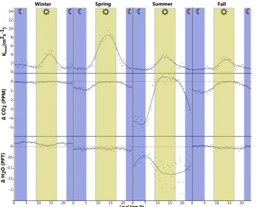
The direction of flux for CO2 can change on a diurnal basis (see Figs. 1 and S3). During the day the flux of CO2is often negative (i.e., downward) due to photosynthe-sis while during the night, plant respiration produces CO2 and fluxes are positive (i.e.
20
to the atmosphere). In addition, atmospheric conditions during the night are typically much more stable than during the day, resulting in a lack of large turbulent eddies and a higher contribution of additional transport mechanisms, such as horizontal advection, to the total flux. The result is that fluxes measured using EC during the night are often underestimated (Aubinet, 2008).
25
ACPD
15, 32759–32777, 2015Comparison of eddy covariance and modified Bowen ratio
methods
D. J. Bolinius et al.
Title Page
Abstract Introduction
Conclusions References
Tables Figures
◭ ◮
◭ ◮
Back Close
Full Screen / Esc
Printer-friendly Version Interactive Discussion
Discussion
P
a
per
|
Discussion
P
a
per
|
Discussion
P
a
per
|
Discussion
P
a
per
|
set from 9 a.m. to 5 p.m. LT. The nighttime/daytime divisions were selected based on the shortest interval between sunrise and sunset at the site. The 8 h periods representing day and night allowed us to construct 24 h, 3 day and 1 week sampling periods by averaging a whole number of 8 h periods taken at the same time of day over multiple days. In addition to the nighttime/daytime split data, we also examined the performance
5
of the MBR method relative to the EC method when using continuous data that ignored day/night differences.
3 Results
3.1 Kheatand concentration gradients
Our calculatedKheat values (Fig. 1) are in good agreement with values for the same
10
site during the same time of year in 2003 (Choi et al., 2008; shown in Fig. S4). Values are close to 0 during the night and in the range of 0.0026 to 35.8 m2s−1during the day over the summer period, with 95 % of the values between 0.029 and 22.11 m2s−1.
The fluxes calculated with the MBR method are proportional to the product ofKheat
and the concentration gradient of either CO2 or H2O (Eq. 1). The raw data at 30 min
15
time resolution that was pooled and used to calculate the fluxes with the MBR method is visualized in Fig. 1.
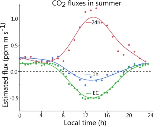
3.2 Performance of the MBR method on continuous time series
When used with continuous time series, fluxes measured with the MBR method are often not of the right magnitude and/or direction for CO2relative to the “reference” EC
20
data (see a representative example in Fig. 2). Inspection of the results indicated that the MBR method would fail when the direction of the flux of CO2 changed during the simulated sampling period. Based on this result, we focused our analysis on comparing the performance of the MBR method to the EC method only during the day or only during the night when fluxes are generally unidirectional.
ACPD
15, 32759–32777, 2015Comparison of eddy covariance and modified Bowen ratio
methods
D. J. Bolinius et al.
Title Page
Abstract Introduction
Conclusions References
Tables Figures
◭ ◮
◭ ◮
Back Close
Full Screen / Esc
Printer-friendly Version Interactive Discussion
Discussion
P
a
per
|
Discussion
P
a
per
|
Discussion
P
a
per
|
Discussion
P
a
per
|
3.3 Performance of the MBR method with hourly-resolved and fixed values of
Kheat
The use of either hourly-resolved data for Kheat or a fixed value did not significantly affect the the MBR method. A studentt test comparing the similarity of the 2 datasets resulted in aP value below 0.0001.
5
Results using a fixed value for Kheat are shown in Table 1; those using hourly-resolved data for Kheat are given in the Supplement (see Table S2).
3.4 Performance of the MBR method on day/night split data
Fluxes of CO2during the nighttime only, measured using the MBR method in combina-tion with simulated sampling times ranging from 1 h to 1 week are on average a factor
10
of 1.7 and up to a factor of 2.1 larger than those derived with the EC method (see Ta-ble 1). Fluxes of CO2during the daytime only, measured using the MBR method have, in some cases, the opposite sign of the fluxes reported using the EC technique. Specifi-cally, the MBR method produces daytime fluxes with the opposite sign compared to the EC method during daytime in the spring and for the 1 week duration simulated
sam-15
pling scenario in the winter (values marked with (!) in Table 1). In those cases where the direction of flux calculated with the MBR does not agree with the EC method, the disagreement is attributable to the median value of∆CO2(between 41.5 and 33 m) se-lected to represent the sampling period having a sign that implies a flux in the opposite direction of the flux measured with the EC method.
20
In cases where the direction of daytime flux measured using the MBR method agreed with the EC method, the ratio of the two fluxes ranged from 0.32 to 1.4, implying that the two methods differed by factors that range from 1.4 to 3.0 and that the MBR method may either underestimate or overestimate fluxes relative to the EC method.
For H2O, the fluxes measured with the MBR method are in the same direction as
25
mea-ACPD
15, 32759–32777, 2015Comparison of eddy covariance and modified Bowen ratio
methods
D. J. Bolinius et al.
Title Page
Abstract Introduction
Conclusions References
Tables Figures
◭ ◮
◭ ◮
Back Close
Full Screen / Esc
Printer-friendly Version Interactive Discussion
Discussion
P
a
per
|
Discussion
P
a
per
|
Discussion
P
a
per
|
Discussion
P
a
per
|
sured by the MBR method to the EC method is between 0.9 and 0.052, implying dif-ferences between the methods by factors of 1.1 to 20, and that fluxes of H2O are underestimated if the MBR method is applied as compared to the EC method. Fluxes measured during the winter season with the MBR method are negative (i.e., from the atmosphere to the surface), while the EC method indicates fluxes are positive (i.e., from
5
the surface to the atmosphere). Fluxes measured by both methods during the night in the fall are small, with a upward flux measured using the EC method and downward fluxes measured by the MBR method in all cases except the longest 1 week simulated sampling period.
In general, the fluxes measured using the two different methods are in better
agree-10
ment for CO2 than for H2O (Table 1). It is interesting to note that the MBR method generally overestimates the flux of CO2 relative to the EC method, while it in most cases underestimates fluxes of H2O.
4 Discussion
The MBR method fails for CO2when using continuous time series in cases where the
15
simulated sampling period encompasses the shift between night and day and there is also a shift from upward fluxes (dominated by respiration) at night to downward fluxes (dominated by photosynthesis) during daytime. As shown in Eq. (3), the flux estimated using the MBR method only depends onKheat and the vertical concentration gradient for the compound of interest. The error arises because the average values ofKheat are
20
dominated by high values that occur during the day, while average values of∆CO2are dominated by extreme values that occur at night (see especially the summer season for CO2in Fig. 1 and data for CO2in the summer visualized in Fig. S5).
The CO2fluxes determined using the MBR method during the daytime for the spring season and when simulating a sampling time of 1 week during daytime for the winter
25
ACPD
15, 32759–32777, 2015Comparison of eddy covariance and modified Bowen ratio
methods
D. J. Bolinius et al.
Title Page
Abstract Introduction
Conclusions References
Tables Figures
◭ ◮
◭ ◮
Back Close
Full Screen / Esc
Printer-friendly Version Interactive Discussion
Discussion
P
a
per
|
Discussion
P
a
per
|
Discussion
P
a
per
|
Discussion
P
a
per
|
development of leaves and the start of photosynthesis taking place halfway accross the season, which would produce a shift from a continuous net flux of CO2 out of the canopy to a diel cycle of CO2uptake and release. Furthermore, it is possible that the simulated 1 week sampling duration during daytime in the winter might have encom-passed periods when the net direction of flux of CO2changed due to the movement of
5
air masses with variable CO2concentrations across the region. Thus, all of the cases of disagreement between the MBR method and the EC method about the direction of flux of CO2that are shown in Table 2 might be attributable to applying the MBR method using simulated sampling times that encompass a change of direction of the net flux.
In general, the duration of simulated sampling does not have a strong influence on
10
the fluxes measured with the MBR method. Exceptions are the longest simulated sam-pling times in during the daytime in winter for CO2 and during nighttime in the fall for H2O. We simulated sampling times of 24 h, 3 days and 1 week by combining data that were measured over non-consecutive 8 h periods during 2 month time windows selected to represent the four seasons. For the 3 day and 1 week simulated sampling
15
times there are just 3 to 4 data-points per season, depending on the data availability, which may introduce higher uncertainty in the median value used in our MBR method calculations compared to the shorter simulated sampling times.
For H2O, which nearly always has a net flux upwards from the canopy during both the day and the night, pooling of the data over longer time intervals and application of
20
the MBR method also led to estimations of the direction of flux that were opposite the EC method in the winter and fall seasons. In winter, fluxes of H2O measured by the EC method were small and upwards, while those calculated with the MBR method were small and downwards (Table 2). A recent study focusing on drainage basins in Canada, reported low but positive fluxes of water vapour during the winter season (Wang et al.,
25
ACPD
15, 32759–32777, 2015Comparison of eddy covariance and modified Bowen ratio
methods
D. J. Bolinius et al.
Title Page
Abstract Introduction
Conclusions References
Tables Figures
◭ ◮
◭ ◮
Back Close
Full Screen / Esc
Printer-friendly Version Interactive Discussion
Discussion
P
a
per
|
Discussion
P
a
per
|
Discussion
P
a
per
|
Discussion
P
a
per
|
while for the MBR method we have used a gradient of concentrations measured at 41.5 and 33 m. During the winter for H2O there was a clear discrepancy between gradients measured at these heights and between 33 and 25.7 m, with the latter being more consistent with the EC measurements (Fig. S6). The cold and low humidity during the winter in Canada might play a role here as discrepancies between the concentration
5
gradients of H2O at different heights were only observed in the winter and to a lesser extent in the fall.
It is clear from our analysis that a requirement for the MBR method to give accu-rate results for prolonged sampling times is to only sample during a time period when the chemicals of interest are expected to have a unidirectional flux. The occurrence
10
of a day/night regime has implications for designing sampling campaigns for organic pollutants that require sampling times longer than the 8 h intervals with stable condi-tions chosen as daytime or nighttime above, and which may exhibit changes in the direction of flux between daytime and nightime periods. This can be the case for many POPs, and the direction of fluxes can be estimated using appropriately parameterized
15
dynamic chemical multimedia fate models (see, for example, Gasic et al., 2010). When longer sampling times are needed, samples could be pooled by sampling at the same time of day during consecutive 24 h periods as was simulated here by combining data from selected 8 h periods.
When sampling over time periods of several hours to several days, as simulated
20
in this study, it is very likely that steady-state conditions during the sampling period are not achieved. Our results indicate however that when fluxes were unidirectional, measurements using the MBR method were usually within 1 order of magnitude of those from the EC method, and that in most cases the difference was less than a factor of 4. The summer period, in which Kheat is low and the gradients of CO2 and H2O
25
ACPD
15, 32759–32777, 2015Comparison of eddy covariance and modified Bowen ratio
methods
D. J. Bolinius et al.
Title Page
Abstract Introduction
Conclusions References
Tables Figures
◭ ◮
◭ ◮
Back Close
Full Screen / Esc
Printer-friendly Version Interactive Discussion
Discussion
P
a
per
|
Discussion
P
a
per
|
Discussion
P
a
per
|
Discussion
P
a
per
|
which is within the range of agreement we obtained between the MBR method and the EC method.
Fluxes measured with the MBR method corresponded better with the EC data for CO2 than for H2O, the reason of which is unknown. However our investigation of the discrepancy in direction of flux between the two methods for H2O in the winter
sug-5
gests that the concentration gradient of H2O is more variable over height than that of CO2. Therefore the gradient that we selected between 41.5 and 33 m may be more representative of the flux measured at 33.3 m with the EC method for CO2 than for H2O.
In general, the variation between fluxes determined using the MBR method for
dif-10
ferent sampling frequencies was small, suggesting that longer sampling times did not introduce a higher bias relative to EC measurements. Using a single value for Kheat, in this case the geometric mean across the sampling period, was found to be a good substitute for hourlyKheat values, indicating that it is possible to use the MBR method when there is no high frequency data available for the transfer coefficient.
15
Some studies have shown that additional transport mechanisms aside from eddy dif-fusion, such as advection, can become more important during night, thereby violating the conditions needed for EC measurements to take place, and resulting in underesti-mations of the night time fluxes (Aubinet, 2008). In this study, there is no clear diff er-ence in the performance of the two methods relative to one another during either day
20
or night. We note however that the MBR method relies onKheat determined under the assumption that only turbulent atmospheric processes occur, so the effect of additional transport mechanisms might not be evident in our analysis.
Based on the findings in this study it is clear that field studies that use the MBR method to measure gas fluxes of POPs and other organic micropollutants should be
25
ACPD
15, 32759–32777, 2015Comparison of eddy covariance and modified Bowen ratio
methods
D. J. Bolinius et al.
Title Page
Abstract Introduction
Conclusions References
Tables Figures
◭ ◮
◭ ◮
Back Close
Full Screen / Esc
Printer-friendly Version Interactive Discussion
Discussion
P
a
per
|
Discussion
P
a
per
|
Discussion
P
a
per
|
Discussion
P
a
per
|
value for the transfer coefficient instead of hourly data is a good alternative that should not introduce a significant bias when there is no high frequency data available. The MBR method could be used to measure fluxes of POPs in depositional areas such as forests as shown by the study of Choi et al. (2008) or in source areas such as large cities where recent studies of vertical concentration gradients of POPs did not lead to
5
quantitative flux estimates (Li et al., 2009; Moreau-Guigon et al., 2007).
The Supplement related to this article is available online at doi:10.5194/acpd-15-32759-2015-supplement.
Author contributions. M. MacLeod had the idea for this study, D. J. Bolinius and M. MacLeod designed the study and D. J. Bolinius gathered the data, performed the analysis and prepared
10
the manuscript with contributions from A. Jahnke and M. MacLeod.
Acknowledgements. We thank Frank Wania for constructive suggestions during the early phases of this work. This research was funded by the Swedish Research Council Vetenskap-srådet (VR), project number 2011-3890, “Investigating thermodynamic controls on the cycling of persistent organic chemicals in forest systems”.
15
References
Aubinet, M.: Eddy covariance CO2 flux measurements in nocturnal conditions: an analysis of
the problem, Ecol. Appl., 18, 1368–1378, doi:10.1890/06-1336.1, 2008.
Baldocchi, D. D., Hincks, B. B., and Meyers, T. P.: Measuring biosphere–atmosphere ex-changes of biologically related gases with micrometeorological methods, Ecology, 69, 1331,
20
doi:10.2307/1941631, 1988.
ACPD
15, 32759–32777, 2015Comparison of eddy covariance and modified Bowen ratio
methods
D. J. Bolinius et al.
Title Page
Abstract Introduction
Conclusions References
Tables Figures
◭ ◮
◭ ◮
Back Close
Full Screen / Esc
Printer-friendly Version Interactive Discussion
Discussion
P
a
per
|
Discussion
P
a
per
|
Discussion
P
a
per
|
Discussion
P
a
per
|
Choi, S.-D., Staebler, R. M., Li, H., Su, Y., Gevao, B., Harner, T., and Wania, F.: Depletion of gaseous polycyclic aromatic hydrocarbons by a forest canopy, Atmos. Chem. Phys., 8, 4105–4113, doi:10.5194/acp-8-4105-2008, 2008.
Gasic, B., MacLeod, M., Scheringer, M., and Hungerbuhler, K.: Assessing the impact of weather events at mid-latitudes on the atmospheric transport of chemical pollutants
us-5
ing a 2-dimensional multimedia meteorological model, Atmos. Environ., 44, 4489–4496, doi:10.1016/j.atmosenv.2010.07.016, 2010.
Gusev, A., MacLeod, M., and Bartlett, P.: Intercontinental transport of persistent organic pol-lutants: a review of key findings and recommendations of the task force on hemispheric transport of air pollutants and directions for future research, Atmospheric Pollut. Res., 3,
10
463–465, doi:10.5094/APR.2012.053, 2012.
Hung, H., MacLeod, M., Guardans, R., Scheringer, M., Barra, R., Harner, T., and Zhang, G.: Toward the next generation of air quality monitoring: persistent organic pollutants, Atmos. Environ., 80, 591–598, doi:10.1016/j.atmosenv.2013.05.067, 2013.
Li, Y., Zhang, Q., Ji, D., Wang, T., Wang, Y., Wang, P., Ding, L., and Jiang, G.: Levels and vertical
15
distributions of PCBs, PBDEs, and OCPs in the atmospheric boundary layer: observation from the Beijing 325-m meteorological tower, Environ. Sci. Technol., 43, 1030–1035, 2009. Majewski, M. S.: Micrometeorologic methods for measuring the post-application volatilization
of pesticides, Water Air. Soil Pollut., 115, 83–113, doi:10.1023/A:1005297121445, 1999. McKone, T. E. and MacLeod, M.: Tracking multiple pathways of human exposure to
persis-20
tent multimedia pollutants: regional, continental and global-scale models, Annu. Rev. Env. Resour., 28, 463–492, doi:10.1146/annurev.energy.28.050302.105623, 2003.
Meyers, T. P., Hall, M. E., Lindberg, S. E., and Kim, K.: Use of the modified bowen-ratio tech-nique to measure fluxes of trace gases, Atmos. Environ., 30, 3321–3329, doi:10.1016/1352-2310(96)00082-9, 1996.
25
Moreau-Guigon, E., Motelay-Massei, A., Harner, T., Pozo, K., Diamond, M., Chevreuil, M., and Blanchoud, H.: Vertical and temporal distribution of persistent organic pollutants in Toronto. 1. Organochlorine pesticides, Environ. Sci. Technol., 41, 2172–2177, doi:10.1021/es062705s, 2007.
Nizzetto, L., Macleod, M., Borgå, K., Cabrerizo, A., Dachs, J., Guardo, A. D., Ghirardello, D.,
30
ACPD
15, 32759–32777, 2015Comparison of eddy covariance and modified Bowen ratio
methods
D. J. Bolinius et al.
Title Page
Abstract Introduction
Conclusions References
Tables Figures
◭ ◮
◭ ◮
Back Close
Full Screen / Esc
Printer-friendly Version Interactive Discussion
Discussion
P
a
per
|
Discussion
P
a
per
|
Discussion
P
a
per
|
Discussion
P
a
per
|
present, and future controls on levels of persistent organic pollutants in the global environ-ment, Environ. Sci. Technol., 44, 6526–6531, doi:10.1021/es100178f, 2010.
Pierce, A. M., Moore, C. W., Wohlfahrt, G., Hörtnagl, L., Kljun, N., and Obrist, D.: Eddy co-variance flux measurements of gaseous elemental mercury using Cavity Ring-Down Spec-troscopy, Environ. Sci. Technol., 49, 1559–1568, doi:10.1021/es505080z, 2015.
5
Stockholm Convention: Stockholm convention on Persistent Organic Pollutants (POPs)
as amended in 2009, available at: http://chm.pops.int/TheConvention/Overview/
TextoftheConvention/tabid/2232/Default.aspx (last access: November 2015), 2010.
Wang, S., Huang, J., Li, J., Rivera, A., McKenney, D. W., and Sheffield, J.: Assessment of water budget for sixteen large drainage basins in Canada, J. Hydrol., 512, 1–15,
10
ACPD
15, 32759–32777, 2015Comparison of eddy covariance and modified Bowen ratio
methods
D. J. Bolinius et al.
Title Page
Abstract Introduction
Conclusions References
Tables Figures
◭ ◮
◭ ◮
Back Close
Full Screen / Esc
Printer-friendly Version Interactive Discussion
Discussion
P
a
per
|
Discussion
P
a
per
|
Discussion
P
a
per
|
Discussion
P
a
per
|
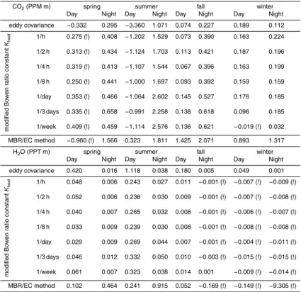
Table 1.Cumulative fluxes for 8 h periods representing day and night across the 2 month peri-ods representing spring, summer, fall and winter. Fluxes measured by the MBR method that are in the opposite direction than those measured by the EC method are marked with “!”. Positive fluxes are defined as fluxes moving upwards from the canopy. The ratio of MBR results over EC results is based on the geometric mean of the MBR results divided by the EC result. The MBR fluxes for the 1 week sampling period were left out in the calculation of the geometric mean during the day in winter for CO2and during the night in fall for H2O. This table shows fluxes
calculated with a constant value forKheat.
CO2(PPM m) spring summer fall winter
Day Night Day Night Day Night Day Night
eddy covariance −0.332 0.295 −3.360 1.071 0.074 0.227 0.189 0.112
modified
Bo
w
en
ratio
constant
Kheat
1/h 0.275 (!) 0.408 −1.202 1.529 0.073 0.390 0.163 0.224
1/2 h 0.313 (!) 0.434 −1.124 1.703 0.113 0.421 0.187 0.196
1/4 h 0.319 (!) 0.413 −1.107 1.544 0.067 0.396 0.163 0.199
1/8 h 0.250 (!) 0.441 −1.000 1.697 0.093 0.392 0.159 0.159
1/day 0.353 (!) 0.466 −1.064 2.602 0.145 0.527 0.176 0.185
1/3 days 0.335 (!) 0.658 −0.991 2.258 0.138 0.618 0.096 0.185
1/week 0.409 (!) 0.459 −1.114 2.576 0.136 0.621 −0.019 (!) 0.032
MBR/EC method −0.960 (!) 1.566 0.323 1.811 1.425 2.071 0.893 1.317
H2O (PPT m) spring summer fall winter
Day Night Day Night Day Night Day Night
eddy covariance 0.420 0.016 1.118 0.038 0.180 0.005 0.049 0.001
modified
Bo
w
en
ratio
constant
Kheat
1/h 0.048 0.006 0.243 0.027 0.011 −0.001 (!) −0.007 (!) −0.009 (!)
1/2 h 0.052 0.006 0.236 0.030 0.009 −0.001 (!) −0.007 (!) −0.008 (!)
1/4 h 0.040 0.007 0.265 0.032 0.008 −0.001 (!) −0.006 (!) −0.007 (!)
1/8 h 0.033 0.009 0.239 0.030 0.008 −0.001 (!) −0.008 (!) −0.008 (!)
1/day 0.029 0.009 0.269 0.044 0.007 −0.001 (!) −0.004 (!) −0.011 (!)
1/3 days 0.046 0.012 0.332 0.050 0.010 −0.003 (!) −0.015 (!) −0.015 (!)
1/week 0.061 0.007 0.323 0.038 0.014 0.001 −0.009 (!) −0.014 (!)
ACPD
15, 32759–32777, 2015Comparison of eddy covariance and modified Bowen ratio
methods
D. J. Bolinius et al.
Title Page
Abstract Introduction
Conclusions References
Tables Figures
◭ ◮
◭ ◮
Back Close
Full Screen / Esc
Printer-friendly Version Interactive Discussion
Discussion
P
a
per
|
Discussion
P
a
per
|
Discussion
P
a
per
|
Discussion
P
a
per
|
-.2 -.15 -0.1 -.05 .0 -5
-4
-3
-2
-1 0
Winter Spring Summer
0 2 4 6 8 10 12 14
∆
FCO
2
F(PPM)
∆
FH
2
OF
(PPT
)
0 5 10 15 20 0 5 10 15 20 0 5 10 15 20 0 5 10 15 20
LocalFtimeF(h) Kheat
(m
2s-1
)
Fall
Figure 1.Half-hourly averages ofKheatand the concentration gradients of CO2and H2O across
ACPD
15, 32759–32777, 2015Comparison of eddy covariance and modified Bowen ratio
methods
D. J. Bolinius et al.
Title Page
Abstract Introduction
Conclusions References
Tables Figures
◭ ◮
◭ ◮
Back Close
Full Screen / Esc
Printer-friendly Version Interactive Discussion
Discussion
P
a
per
|
Discussion
P
a
per
|
Discussion
P
a
per
|
Discussion
P
a
per
|
CO28fluxes8in8summer
E
st
ima
te
d
8f
lu
x8
(p
p
m8
m8
s-1)
Local8time8(h)
1.0
0.5
0.0
-0.5
0 4 8 12 16 20 24
24h
1h
EC
Figure 2.A comparison of measured fluxes using the modified Bowen ratio (MBR) method (1 and 24 h pooled data using hourlyKheat values) with the eddy covariance (EC) measurements. The simulated 24 h sampling time includes a change in the direction of the CO2 flux, which