www.hydrol-earth-syst-sci.net/16/1095/2012/ doi:10.5194/hess-16-1095-2012
© Author(s) 2012. CC Attribution 3.0 License.
Earth System
Sciences
Turbulent flux modelling with a simple 2-layer soil model and
extrapolated surface temperature applied at Nam Co Lake
basin on the Tibetan Plateau
T. Gerken1,2, W. Babel2, A. Hoffmann1, T. Biermann2, M. Herzog1, A. D. Friend3, M. Li4, Y. Ma5, T. Foken2,6, and H.-F. Graf1
1Centre for Atmospheric Science, Department of Geography, University of Cambridge, UK 2Department of Micrometeorology, University of Bayreuth, Germany
3Department of Geography, University of Cambridge, UK
4Cold and Arid Region Environmental and Engineering Research Institute, Chinese Academy of Sciences, Lanzhou, China 5Institute of Tibetan Plateau Research, Chinese Academy of Sciences, Beijing, China
6Member of Bayreuth Center of Ecology and Environmental Research (BayCEER), University of Bayreuth, Germany
Correspondence to:T. Gerken ([email protected])
Received: 19 October 2011 – Published in Hydrol. Earth Syst. Sci. Discuss.: 21 November 2011 Revised: 8 March 2012 – Accepted: 27 March 2012 – Published: 3 April 2012
Abstract. This paper introduces a surface model with two soil-layers for use in a high-resolution circulation model that has been modified with an extrapolated surface temperature, to be used for the calculation of turbulent fluxes. A quadratic temperature profile based on the layer mean and base tem-perature is assumed in each layer and extended to the sur-face. The model is tested at two sites on the Tibetan Plateau near Nam Co Lake during four days during the 2009 Mon-soon season. In comparison to a two-layer model without ex-plicit surface temperature estimate, there is a greatly reduced delay in diurnal flux cycles and the modelled surface tem-perature is much closer to observations. Comparison with a SVAT model and eddy covariance measurements shows an overall reasonable model performance based on RMSD and cross correlation comparisons between the modified and original model. A potential limitation of the model is the need for careful initialisation of the initial soil temperature profile, that requires field measurements. We show that the modified model is capable of reproducing fluxes of similar magnitudes and dynamics when compared to more complex methods chosen as a reference.
1 Introduction
Turbulent fluxes of momentum, latent heat (QE) and
sensi-ble heat (QH) are some of the most important interactions
between land surface and atmosphere. These fluxes are re-sponsible for the development or modification of mesoscale circulations and the generation of clouds feed back on sur-face fluxes through the modification of solar radiation. The effects of vegetation influencing boundary layer structure and moisture are widely acknowledged (i.e. Freedman et al., 2001; van Heerwaarden et al., 2009), while the feedback from short-lived clouds is less understood, but important. Shallow cumulus-surface interactions were shown in an LES (large eddy simulation) study to impact surface tempera-ture and fluxes on very short time scales (Lohou and Patton, 2011). For improved process understanding, it is necessary to use: (1) atmospheric models with sufficiently high resolu-tion (O(100 m)) to resolve boundary layer processes as well
as clouds and (2) surface models capable of reproducing the system’s surface flux dynamics.
include large temporal and spatial variability in soil mois-ture (Su et al., 2011), large diurnal variations of surface tem-perature from surface freezing before sunrise to more than 30◦C at noon. Ma et al. (2009) give an overview about the
TP surface-atmosphere processes. On the TP, the fraction of diffuse solar radiation is very small, making cloud feed-backs especially important for the surface-atmosphere sys-tem. The model studies with a regional model of Cui et al. (2007) imply that some of the precipitation events on the TP are predominantly local and therefore not captured by coarser resolution models.
In this paper we present results of a rather simple flux algorithm based on a modified two-layer soil model that is part of a vegetation dynamics and biosphere model Hybrid (Friend et al., 1997; Friend and Kiang, 2005; Friend, 2010). The original model produces a substantial delay in the di-urnal turbulent flux cycle due to the low responsiveness of the model’s upper soil layer to changes in atmospheric forc-ing and fails to capture important dynamics. We therefore introduce an extrapolated surface temperature and show that this new approach is capable of reproducing diurnal flux dy-namics for two vegetation covered surfaces near Nam Co Lake. These sites are representative for the basin, but show very different dynamics. In our future studies, the same surface-model version will also be coupled to the spatially and temporally high resolution atmospheric model ATHAM (Active Tracer High-resolution Atmospheric Model, Ober-huber et al., 1998; Herzog et al., 1998) including radiation, cloud microphysics and active tracer transport. As simula-tions of the high-resolution model will be run for approx-imately 24 h we tested the surface model in column mode forced with standard atmospheric measurements for the same period of time with initialisation at 00:00 h Beijing Standard Time (BST). We acknowledge that this approach is different from most surface model studies that are run for longer peri-ods, but it is necessary for the planned study of the coupled surface-atmosphere system. Such a surface flux algorithm is generally suitable for high-resolution atmospheric modelling studies of different ecosystems as it does not have built in assumptions about horizontal scales.
It is our objective to test the suitability of a simple two-layer soil model with an improved surface or “skin” tem-perature estimated from the mean temtem-perature of the upper-most layer that shall subsequently be used for driving an at-mospheric circulation model for the Nam Co region on the TP. Therefore, fluxes derived from the surface flux algorithm with and without a specific formulation for “skin” temper-ature are compared to fluxes measured by eddy-covariance technique and to fluxes derived by a more complex Surface-Vegetation-Atmosphere Transfer (SVAT) Model, with five soil layers.
E
E
E NamITP
E NamUBT
Nam Co building grass(+) grass(-) gravel lake wetland
0 500 1,000 2,000 3,000
Meters
Fig. 1. Landcover map of study area: the black cross indicates the station identified as UBT, close to the small lake with denser surface cover [grass (+)], the red cross shows the station location ITP with sparse surface cover [grass (-)].
2 Site description and model forcing data
From 27 June to 8 August by the University of Bayreuth (UBT) and the Institute of Tibetan Plateau Research, Chinese Academy of Sciences (ITP) conducted a joint field campaign at Nam Co Lake.
2.1 Site description
Nam Co Lake is located on the Tibetan Plateau at approxi-mately 4730 m a.s.l., circa 150 km north of Lhasa. Data from two locations in the vicinity of the lake are used (Fig. 1). Site 1, referred to and operated by UBT, is an eddy-covariance setup on the south shore of a small lake that itself is situ-ated approximately 500 m south of Nam Co lake. UBT has a fairly constant soil moisture below circa 60 cm depth due to the influence of ground water. Additionally, the atmospheric measurements are influenced by a land-lake breeze that orig-inates from Nam Co Lake. Site 2 (operated by and referred to as ITP) is at the Nam Co Station for Multisphere Observa-tion and Research (Li et al., 2009; Cong et al., 2009), approx-imately 300 m south from both UBT and the direct influence of the small lake with a sandy soil and a very low field capac-ity (FC = 5 %) compared to overall pore volume (39 %). The vegetation at both sites is grassland (Metzger et al., 2006) with UBT having a small bare soil fraction (0.1) compared to 0.4 at ITP). Small FC and the generally low volumetric top soil water contents (θv) at ITP, lead to large sensible
en-ergy fluxes compared to latent heat fluxes (QH≫QE).
Af-ter rain events however, θv may exceed FC by a factor of
up to 3 leading to a similar flux regime at the two stations withQE> QH. Due to the generally drier conditions,
00:00 06:00 12:00 18:00 00:00
0 400 800
1200 a) SW
[W m
−2
]
10−Jul 27−Jul 05−Aug 06−Aug
00:00 06:00 12:00 18:00 00:00
200 250 300 350 400
b) LW
[W m
−2
]
2 6 10
14 c) T
[
° C]
7 8 9 10
d) q
[g kg
−1 ]
00:00 06:00 12:00 18:00 00:00
2.5 5 7.5
10 e) u
[m s
−1
]
0 1 2
[mm (0.5h)
−1
]
00:00 06:00 12:00 18:00 00:00
572.5 575 577.5
f) P + Precip
[hPa]
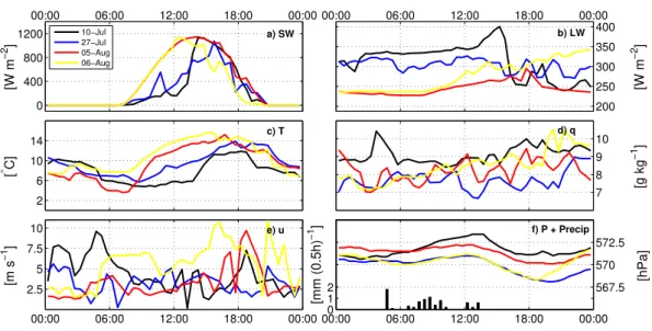
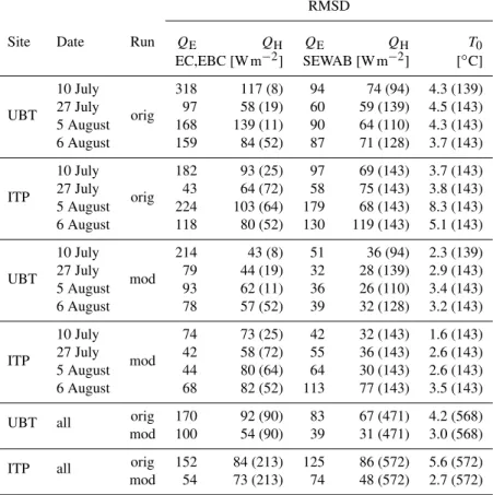
Fig. 2. Forcing data measured at UBT used for model runs:(a)downward shortwave radiation (SW [W m−2]); b) downward longwave radiation (LW[W m−2]);(c)air temperature (T [◦C]);(d)water vapour mixing ratio (q[g kg−1]);(e)wind speed (U[m s−1]);(f)surface pressure (P [hPa]) and precipitation [mm(0.5h)−1]) Height c–e is 3 m.
frequently drops below 0◦C in the early morning hours. At UBT there were soil temperature sensors installed at 2.5, 5, 10, 20, 30 and 50 cm depths. At ITP no soil temperatures were available at depths above 20 cm, with data measured at 20, 40, 80 and 160 cm below ground. Comprehensive infor-mation of ITP and UBT surface and soil properties, measure-ment setup and data availability is found in (Biermann et al., 2009) and an overview over the parameters used in the model is presented in Table 1.
2.2 Model forcing data
The data used in the modelling study was selected accord-ing to the data quality of turbulence data (Foken et al., 2004) and the wind direction. Finally, we selected four days with high data quality over the whole day encompassing different weather situation. The 24-h model runs are initialised with the soil temperature profile and soil moisture at 00:00 BST (∼22:00 in local solar time). 10 July was a complex day with rain in the morning and sunshine in the afternoon. 27 July was a cloudy day without rain. 5 August was a radiation day after a period of rain leading to moist conditions and large
QEat ITP. 6 August was similar to the previous day, but with
some of the water drained from the soil at ITP and develop-ing clouds in the afternoon. Durdevelop-ing 10 July and 5 August, the station close to the lake (UBT) came under the influence of a lake breeze during which the forcing data (except for ra-diation measurements) correspond rather to the nearby lake than the land surface. Due to the overcast sky on 27 July the lake breeze and thus the influence of the lake surface was severely weakened as described in Zhou et al. (2011), so that there was only limited influence of the lake surface onto the atmospheric measurements.
The model is forced with measured atmospheric data from UBT (Fig. 2) and ITP (Fig. 3) providing air temperature, wa-ter vapour mixing ratio, wind speed, air pressure, precip-itation and downwelling long and shortwave radiation. In general 30-min mean values were linearly interpolated to the surface model time step that was the same as a typical time step of an atmospheric model (1t=2.5 s). The only selected day with precipitation during day-time was 10 July 2009. However, there was also rain recorded at UBT from about 22:00 BST on 6 August 2009, while no precipitation data was available at ITP. Half hourly precipitation was scaled down to the model time step assuming a constant precipi-tation rate per 30-min interval. There was little difference between the data measured at ITP and UBT, as expected due to the proximity of the sites. However there was an offset of approx. 5 hPa between the recorded pressures, that was not corrected for as this is likely within the uncertainty of the sensors and the model should not be too sensitive to such a pressure difference. Unlike UBT where rain 30-min precipi-tation was available, there were only daily sums recorded for ITP, which had to be downscaled to 30-min values by scaling them linearly with UBT observations.
3 Modelling approach
Table 1.Description of the two sites (UBT and ITP) near Nam Co lake and the parameters used the model setup (Biermann et al., 2009).
Parameter UBT ITP
Coordinates 30
◦46.50′N 30◦46.44′N
90◦57.61′E 90◦57.72′E
Soil sandy-loamy sandy
Porosity 0.63 0.393
Field capacity [m3m−3] 0.184 0.05
Wilting point [m3m−3] 0.115 0.02
Heat capacity of dry soil (cpd) [J m−3K−1] 2.5×10⁶ 2.2×10⁶
Thermal conductivity [W m−1K−1] 0.53 0.20
Surface albedo (α) 0.20 0.20
Surface emissivity (ǫ) 0.97 0.97
Vegetated fraction 0.9 0.6
LAI [m2m−2] (estim. from: Hu et al., 2009) 0.9 0.6
Vegetation height [m] 0.07 0.15
00:00 06:00 12:00 18:00 00:00
0 400 800
1200 a) SW
[W m
−2
]
10−Jul 27−Jul 05−Aug 06−Aug
00:00 06:00 12:00 18:00 00:00
200 250 300 350 400
b) LW
[W m
−2
]
2 6 10
14 c) T
[
° C]
7 8 9 10
d) q
[g kg
−1 ]
00:00 06:00 12:00 18:00 00:00
2.5 5 7.5
10 e) u
[m s
−1
]
0 1 2
[mm (0.5h)
−1
]
00:00 06:00 12:00 18:00 00:00
567.5 570 572.5
f) P + Precip
[hPa]
Fig. 3. Same as Fig. 2, but with forcing data measured at ITP. Precipitation at ITP was measured daily and for the purpose of this study distributed to 30 minute intervals according to the recorded rain fall at UBT.
Our high-resolution modelling approach aims at a spatial and temporal resolution in the order of 500 m and 2.5 s, re-spectively. As our focus is on diurnal surface-atmosphere interactions, the surface model must capture the magnitude of the fluxes and must be able to react quickly to changes in atmospheric forcing. Therefore, a surface model that is capable of reproducing realistic turbulent energy and water vapour fluxes at a sufficiently high temporal resolution and at reasonable computational costs is needed. We decided against a model with more than two soil-layers due to higher computational cost and instead modified the original Hybrid model to meet these requirements.
3.1 The surface model
The modified version of Hybrid which is a process based terrestrial ecosystem and surface model, incorporates a sim-ple two-layer representation of the soil and uses the turbu-lent transfer parameterisations taken from the GISS model II (Hansen et al., 1983). The transfer equations in Hybrid are described in Friend and Kiang (2005). Bare soil param-eterisation follows the approach of SSiB (Xue et al., 1996) that is based on Camillo and Gurney (1986) and Sellers et al. (1986). Turbulent fluxes are calculated using a bulk approach for the sensible heat flux:
QH=cpρ CHu(z) (T0−T (z)) (1)
with air specific heat capacity (cp[J kg−1K−1]), the Stanton
length (z0) and Bulk Richardson Number, air density (ρ
[kg m−3]), measured wind speed (u(z) [m s−1]), air
tem-perature (T (z)) at measurement height (z[m]) and surface temperature (T0). All temperatures used are in K. The
la-tent heat flux is derived in a more complex manner from bulk soil evaporation (EV) and a canopy resistance approach estimating plant transpiration (TR), withQE=EV+TR:
EV=
ρfhqs−qa rs+ra
×exp(−0.7LAI) (2)
TR= ρ1qa
rc+ra
, (3)
with the relative humidity of soil air (fh), saturation water
mixing ratio at surface temperature (qs), atmospheric water
vapour mixing ratio (qa), soil and aerodynamic resistance (rs, ra), leaf area index (LAI) and canopy resistance (rc)
calcu-lated by the vegetation model component. Transfer coeffi-cients are modified from Deardorff (1968). Plant physiol-ogy and stomatal conductance are included via generalised plant types (GPT). As an ecosystem model Hybrid is de-signed to work on hourly to climate scales (Friend, 2010) and and should therefore be capable of reproducing diurnal flux cycles as well as ecosystem changes on climate scales. It was originally developed as a biosphere-surface component for the GISS GCM. A “thin” upper layer of 10 cm thickness follows the daily cycle of surface temperatures, whereas a lower layer with 4 m thickness acts as the memory for the an-nual cycle in both model versions. However, an upper layer of such thickness imposes a substantial dampening on the diurnal temperature cycle and will effectively act as a low-pass filter for events of short durations such as cloud shading that, especially under the conditions found at the TP, has a substantial immediate impact on surface temperatures and on fluxes as well. This can be seen in Fig. 12 of Hansen et al. (1983), where a time delay of approximately 2 h is visible for surface temperature in the diurnal cycle. A similar behaviour of the original Hybrid is discussed in Sect. 5.4. Shortcom-ings with the representation of diurnal cycles may also im-pact on longer term studies as the model drifts away from a realistic state. As we plan to apply the coupled model for high-resolution simulations with a time step in the order of seconds, we focus in this work on the accuracy of the diurnal flux cycles that can be achieved with such a model.
3.2 The modified soil model in Hybrid
In order to improve the delay in diurnal flux evolution and the weak responsiveness of sudden short-term changes in at-mospheric forcing, new simulation approaches for surface temperature and heat diffusion were introduced in Hybrid.
3.2.1 Diagnostic surface temperature
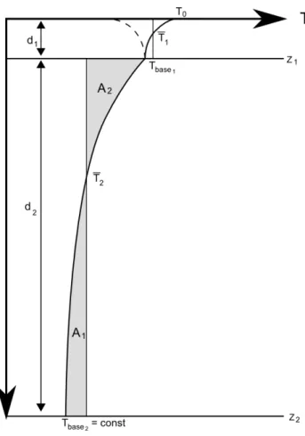
An extrapolated surface temperature (T0) is being introduced
that is then subsequently used for the calculation of
atmo-Fig. 4.Conceptional drawing of the assumed quadratic subgrid soil temperature profile and the associated parameters. In order to derive
¯
T1andT¯2geometrically the areasA1andA2must be equal.
spheric stability through the Bulk Richardson number as well as for QH andQE. This approach is somewhat similar to
the “force-restore method” (Blackadar, 1979) that also aims at providing a realistic surface temperature imitating the be-haviour of real soils. However, while “force-restore” uses an oscillating heat source as forcing term and a heat flux into the ground as restoring term (Yee, 1988), our method is not de-pendent on a periodic heating function and uses the concept of layer heat storage.T0is derived from a set of assumptions
that were already included in Hybrid going back to Hansen et al. (1983). For both layers denoted with the subscripts 1 and 2 from the model top, we assume a quadratic temperature profile (T (z)) (Fig. 4):
T1,2(zrel)=a1,2 zrel−d1,22+Tbase1,2 (4) with a constant (a[K m−2]), the depth below the top of the layer (zrel[m]), the layer thickness (d[m]) and the
temper-ature at the lower boundary of the respective layer (Tbase).
However, the annual temperature cycle at 4 m is expected to be small and the rate of change as well as the diurnal temper-ature cycle is too small to have an impact on the day scale. For future research the seasonal mean temperature could be used in order to remove this potential source of error. The re-lationship between layer heat contentE[J] and temperature profile is given by:
E=cps
zU
Z
zL
T (z)dz (5)
where zL and zU are the lower and upper boundaries of
the layer andcps [J m−
3K−1] is the total soil heat capacity.
Hence, with a known heat content for each layer it is possible to solve for
a2=
E2
cps,2 −d2Tbase2
d23
3
, (6)
by integrating Eq. (5) with Eq. (4) fromzL =0 tozU =d2
and solving fora2. The base temperature of the first layer is
related toTbase2through
Tbase1=Tbase2+a2d2
2. (7)
In a similar fashiona1andT0can be approximated:
a1=
E1
cps,1 −d1Tbase1
−z13
3
(8)
and
T0=Tbase1+a1d1
2.
(9) As Tbase1 is a parameter of both Eqs. (7) and (9) and a1,2 are of crucial importance to the initialisation ofE1,2,
spe-cial care has to be taken, when assigning initial conditions (see discussion in Sect. 3.3).
3.2.2 Heat diffusion estimation
The soil heat flux is derived from the residual of the surface energy balance. In the original heat diffusion algorithm of Hybrid (Hansen et al., 1983), the heat flux from the first to the second soil layer F (z) is dependent on the difference between mean surface layer temperatures (T¯), the soil heat flux calculated as residual of turbulent and radiation fluxes (F (0)), layer thickness and thermal resistancesr,
F (z)=3T¯1−3T¯2−0.5F (0)r1
r1+r2 ×
1t, (10)
where1t is model time-step. This leads to unrealistic mod-elled heat fluxesF (z)asF (z)is largely dominated byF (0), which is positive during nighttime and negative during day-time, thus leading to a net transfer of heat from a cold to
a warm layer. With the assumption of a subgrid tempera-ture profile the heat flux between the two layers Eq. (10) was modified with a heat diffusion approach and integration of
∂T ∂t =D
∂2T ∂z2 ≈D1t
T (z1+1z)−2T (z1)+T (z1−1z)
21z (11)
withD being a soil moisture dependent diffusion constant for heat. We assume ∂z to be approximated by the dif-fusion length L=2√1tD=1z and the temperatures are taken from the assumed profile. As the model is run with the short time-step of the atmospheric model, such a for-mulation becomes valid. A rough calculation for L with
D=10−6m2s−1, which is close to the determined value, and1t =30 min gives L=0.08 m, which is close to d1,
posing an upper limit on1t for this method.
3.3 Surface temperature profile initialisation
Due to the quadratic nature of the soil layer temperature pro-files and their potential kink at the layer interface (see Fig. 4), the modified model depends on careful initialisation that ful-fills two requirements: (1) a realistic estimate of surface tem-perature and (2) an appropriate estimate of ground heat stor-age (E) allowing the upper layer to react in a realistic way. In this study soil temperature measurements at several depths were used in order to accomplish both requirements. Surface temperature was estimated from upwelling longwave radia-tion according to the Stefan-Boltzmann law with a longwave emissivity ofǫ =0.97. We initialisedE2by settingTbase1 to the measured 10 cm temperature and then subsequently fit-ted the temperature curve for the first model layer by min-imising the squared mean error with regard to measured soil temperatures. Due to the lacking 10 cm temperature at ITP, this temperature had to be estimated from the 20 cm mea-surement andT0was approximated in order to estimate the
initial E1. It should be noted that the assumed quadratic
temperature profile in the lower soil layer clearly underes-timated the vertical temperature gradient in the soil as esti-mated UBT temperatures at 50 cm were always higher than measured temperatures. This difference is reduced from July to August as the summer warming reaches lower layers. This is a limitation due to fixed layer depths.
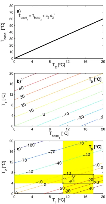
Table 2 shows the initial temperatures for each day. From the span of layer temperaturesT¯1andT¯2, the theoretical
pa-rameter space ofT0for a constantTbase2 (Fig. 5) can be de-rived. While Fig. 5a and b show the individual dependence of temperature variables on each other as expressed in the re-spective Eqs. (7) and (9), Fig. 5c shows the combined effect of parameter variation. A random combination of the initial temperatures given in Table 2 would yieldT0in the rage of
Table 2. Initial soil temperatures used in this study (T¯2andT¯1are estimated from the respective base and top temperatures of the layer according to a quadratic temperature profile), change of layer 1 mean temperature (1T¯1) over the modified Hybrid run, soil moisture content of layer 1 at beginning of the modified model run (θ1obs) and at the end of the simulation (θ1end). The values in parenthesis are expressed as θ1/FC[-].
¯
T2 T1,base T¯1 T0 1T¯1 θ1obs θ1end
Site Date [◦C] [◦C] [◦C] [◦C] [◦C] [%] [%]
UBT
10 July 3.9 11.8 10.9 9.3 −1.6 26.9 (1.47) 41.1(2.24)
27 July 4.5 13.4 12.5 10.6 −1.6 20.8 (1.14) 17.0 (0.92)
5 August 4.8 14.4 13.4 11.2 −3.0 26.9 (1.47) 19.1 (1.04)
6 August 4.75 14.3 12.8 9.8 −1.4 25.4 (1.39) 34.0 (1.85)
ITP
10 July 5.4 16.2 13.2 7.2 −1.2 6.0 (1.1) 25.1 (5.02)
27 July 7.2 21.6 17.8 10.2 −1.7 3.0 (0.6) 1.6 (0.32)
5 August 5.7 17.1 11.1 −0.8 0.2 11.0 (2.2) 4.3 (0.86)
6 August 5.6 16.8 11.6 1.1 1.9 9.0 (1.8) 3.7 (0.73)
about subsurface temperatures that are difficult to estimate without field measurements.
4 Flux comparison
Surface fluxes derived with any method contain inaccura-cies such as measurement errors or theoretical limitations. Therefore we are not comparing our modelling results to the absolute truth, but to two flux references.
4.1 EC and SEWAB reference fluxes
Fluxes estimated by both versions of Hybrid are com-pared with observed fluxes derived by eddy covariance (EC) method and fluxes modelled by the SVAT model SEWAB (Surface Energy and Water Balance model – Mengelkamp et al., 1999), which has been configured for the two sites for gap-filling and up-scaling of flux measurements. Both flux references yield fluxes averaged over 30-min intervals. Un-like many SVAT models that derive the soil heat flux from the flux residual, SEWAB is solving the surface energy bal-ance equation (QE+QH+QRad+QSoil=0) iteratively forT0
by Brent’s method (Mengelkamp et al., 1999), hence closing the energy balance locally (Kracher et al., 2009). In contrast, the surface energy balance closure derived by EC is only in the order of 0.7 at Nam Co Lake (Zhou et al., 2011). Con-sequently, 30 % of the net radiation is not captured by sur-face flux measurements. However, energy balance closure must not be used as a quality measure for flux measurements (Aubinet et al., 1999) as surface heterogeneity leads to or-ganised low frequency structures and mesoscale circulations (Panin et al., 1998; Kanda et al., 2004) that are mainly re-sponsible for the lack of closure (Foken, 2008). The energy balance problem for eddy-covariance measurements is sum-marized in Foken et al. (2011). Additionally, in sea (lake) breeze systems a significant portion of the energy fluxes is transported horizontally (Kuwagata et al., 1994). Therefore,
SEWAB (and Hybrid) fluxes are comparatively larger than the measured ones. When the energy balance is closed artifi-cially by redistributing the residual to fluxes according to the Bowen ratio (Twine et al., 2000), the resulting fluxes are in much better agreement with SEWAB (not shown). Therefore energy balance corrected fluxes are used whenever possible (QEEC,EBCandQHEC,EBC). Artificial energy balance closure is only possible, when the Bowen ratio can be determined from flux measurements and when data about the available energy is measured. EC data were collected at 3 m height and cal-culated using the TK3 package (Mauder et al., 2008; Mauder and Foken, 2011). Quality checks were performed accord-ing to Foken et al. (2004). A detailed description of the in-strumentation can be found in Biermann et al. (2009). The rain event of 10 July leads to the exclusion of fluxes due to quality concerns. Both Hybrid and SEWAB produce fluxes during rain, but their quality is unknown as they cannot be compared to measurements.
Measuring in close proximity to the lake also means that depending on wind direction the fluxes measured at UBT are originating from land, water or a mixture of both as the foot-print of the EC system and thus also of the forcing data is located upwind of the site. This leads to problems in the en-ergy balance closure and the integration of fluxes. The devel-opment of a lake breeze system at Nam Co means that during most days there are no flux measurements available from the late morning or early afternoon until the lake breeze ceases. The days of 27 July and 6 August are the only days during which the field campaign provides data that do not have a full lake breeze influence at UBT. Therefore it is beneficial to compare not only to measured fluxes, but also to SEWAB (QESEWABandQHSEWAB).
0 4 8 12 16 20 0
10 20 30 40 50 60 70 80
T 2 [°C]
T base
1
[
°
C]
a)
Tbase
1
= Tbase
2
+ a2 d22
−30 −20
−10 0
10 20 30 40 50
b) T0 [°C]
T base
1 [°C]
T 1
[
°
C]
0 4 8 12 16 20
0 4 8 12 16 20
0 4 8 12 16 20
0 4 8 12 16 20
−100 −70
−70
−70
−40
−40
−40
−10
−10
−10
0
0
0
0
20
20
30
30 40 c) T0 [°C]
T 1 [°C]
T 2
[
°
C]
Fig. 5. Dependency of soil temperature parameters:(a) relation-ship between mean temperature of layer 2 (T¯2) and bottom tem-perature of layer 1 [Tbase1, Eq. (7)] –a2is calculated according
to Eq. (6);(b)surface temperature (T0) contour plot as function of
Tbase1and layer 1 mean temperature (T¯1) and(c)contours of (T0) as function ofT¯2andT¯1. The black rectangle at the intersection of the layer temperature ranges (yellow) indicates the theoretical parame-ter space given by the temperature values used in this study and the black crosses mark the actual configurations.
4.2 Statistical evaluation measures
Model quality was assessed by Root Mean Square Deviation (RMSD)
RMSD= v u u
t1
N N X
i=1
Pp−Pr 2
i (12)
and Cross Correlation according to the coefficient of determination (R2):
R2(j )= cov Pp(1+j:N ), Pr(1:N−j )
σPp(1+j:N )σPr(1:N−j )
!2
(13)
withR2(j ) being the coefficients of determination for the predicted (Pp) and reference (Pr) flux time series shifted by j elements, the total number of elements in each time se-ries (N) andσ as their respective standard deviations. Both SEWAB and EC measurements produce 30-min flux aver-ages, whereas Hybrid was set to 10-min averaged fluxes. Therefore the reference fluxes were linearly interpolated to Hybrid’s output times before statistical evaluation. Periods when no energy balance corrected EC measurements were available (see Figs. 6 and 7 for details) were excluded from the calculation of the statistical measures.
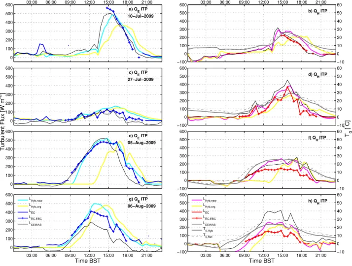
5 Results and discussion
The following section presents and discusses the improve-ments that are achieved for a simple two-layer model when a new algorithm for the surface temperature was implemented. The original two-layer model Hybrid fails to reproduce the diurnal dynamics observed at UBT (Figs. 6 and 7) due to the thermal inertia of the top-layer. The delayed response in face temperature leads to a shift in the resulting turbulent sur-face fluxes. This causes an underestimation ofQEandQH
until∼18:00 BST and later to an overestimation due to de-layed surface cooling. The improvement of the modified Hy-brid over the original formulation is discussed in more detail in Sects. 5.1 and 5.4.
0 100 200 300 400 500 600 a) Q
E UBT
10−Jul−2009
Turbulent Flux [W m
−2
]
03:00 06:00 09:00 12:00 15:00 18:00 21:00
−100 0 100 200 300 400 500 600 b) Q
H UBT
−10 0 10 20 30 40 50 60 T 0 [ °C]
03:00 06:00 09:00 12:00 15:00 18:00 21:00
0 100 200 300 400 500 600 c) Q
E UBT
27−Jul−2009 −100 0 100 200 300 400 500 600 d) Q
H UBT
−10 0 10 20 30 40 50 60 0 100 200 300 400 500 600 e) Q
E UBT
05−Aug−2009 L Hyb,new L Hyb,org WCOARE L EC L EC,EBC LSEWAB −100 0 100 200 300 400 500 600 f) Q
H UBT
−10 0 10 20 30 40 50 60 L Hyb,new L Hyb,org WCOARE L EC L EC,EBC LSEWAB
03:00 06:00 09:00 12:00 15:00 18:00 21:00 0 100 200 300 400 500 600 g) Q
E UBT
06−Aug−2009 Time BST L+W EC W EC WHM −100 0 100 200 300 400 500 600 h) Q
H UBT
−10 0 10 20 30 40 50 60 L+W EC W EC W HM T 0,Hyb T 0,Ref
03:00 06:00 09:00 12:00 15:00 18:00 21:00 Time BST
Fig. 6.Model results for the modified Hybrid at UBT for 10 July 2009(a–b), 27 July 2009(c–d), 5 August 2009(e–f)and 6 August 2009
(g–h). Left column: latent heat flux (QE); right column: sensible heat flux (QH) and surface temperatureT0[◦C].LandWrefer to “land” and “water” as origin of the fluxes.L+Wis the complete available time series. The subscriptsHyb,modandHyb,orgrefer to fluxes from the modified and original Hybrid andCOAREare fluxes from the lake derived by TOGA-COARE whereasSEWABis a SVAT model andHM
refers to a hydrodynamic multi-layer lake model after Foken (1984) and Panin et al. (2006).ECandEC,EBCrefer to measurements by eddy covariance method where in the latter the energy balance has been closed by distributing the residual according to Bowen-ratio (this requires good data quality and fluxes and can only be done for fluxes that are attributed to land). The circles indicate poor data quality of the EC system according to Foken et al. (2004). Gray shading indicates times where the flux footprint of UBT was over the lake.
The situation at ITP is quite similar to UBT. The modi-fied model agrees well with the EC and SEWAB reference data. On 5 August the turbulent flux dynamics, but not the magnitude of the fluxes, match the EC measurements closely (Fig. 7), while the original Hybrid showed a strong delay in the flux response as the soil remained frozen during the morning. While the magnitude of the latent heat flux is close to EC measurements,QH produced by Hybrid are of a
sim-ilar magnitude asQHfrom SEWAB. These are considerably
larger than the fluxes measured by EC and corrected for en-ergy balance closure. For 6 August the modelled maximum ofQEis larger than the maximumQEEC,EBCand much greater throughout most of the day compared to SEWAB.QHin
con-trast shows similar diurnal dynamics asQHEC,EBC, but with its
magnitude between the sensible heat flux derived by SEWAB andQHEC,EBC. Around 18:00 h theQH-fluxes from the differ-ent methods become more similar. A large negativeQH-flux
in the morning hours is apparent but greatly improved com-pared to the unmodified Hybrid version. Figure 6a and b also highlights some limitations of ecosystem research as a large portion of the data had to be rejected due to limitations described in Sect. 4.1.
0 100 200 300 400 500 600 a) Q
E ITP
10−Jul−2009
Turbulent Flux [W m
−2
]
03:00 06:00 09:00 12:00 15:00 18:00 21:00
−100 0 100 200 300 400 500 600 b) Q
H ITP
−10 0 10 20 30 40 50 60 T 0 [ ° C]
03:00 06:00 09:00 12:00 15:00 18:00 21:00
0 100 200 300 400 500 600 c) Q
E ITP
27−Jul−2009 −100 0 100 200 300 400 500 600 d) Q
H ITP
−10 0 10 20 30 40 50 60 0 100 200 300 400 500 600 e) Q
E ITP
05−Aug−2009 −100 0 100 200 300 400 500 600 f) Q
H ITP
−10 0 10 20 30 40 50 60
03:00 06:00 09:00 12:00 15:00 18:00 21:00 0 100 200 300 400 500 600 g) Q
E ITP
06−Aug−2009 Time BST L Hyb,new LHyb,org L EC L EC,EBC LSEWAB −100 0 100 200 300 400 500 600 h) Q
H ITP
−10 0 10 20 30 40 50 60 L Hyb,new LHyb,org L EC L EC,EBC LSEWAB T 0,Hyb T 0,Ref
03:00 06:00 09:00 12:00 15:00 18:00 21:00 Time BST
Fig. 7.Same as Fig. 6, but for ITP. There are no contributions from the lake.
and 6 August. On 5 August there is at least a qualitative agreement between COARE and EC measurements.
5.1 Discussion of turbulent fluxes
The original two layer model reacts only slowly to the atmo-spheric forcing, delaying the fluxes’ response. Such a time lag leads to a shift in the diurnal cycle and is problematic for the coupling to atmospheric models since surface fluxes are one of the main drivers of regional and local circulation as well as cloud development. These will certainly be affected by erroneous surface flux dynamics. In our specific case, the dampening of the diurnal temperature cycle and the delay in surface fluxes may reduce the intensity of the land-lake breeze or may delay its development through a reduction of differential heating between land and lake surface. However, there is still a minor delay visible in the modified Hybrid as the surface temperature is purely diagnostic and dependent onT¯1. This is discussed in more detail in Sect. 5.4.
Table 3 shows the results of the RMSD between the mod-elled results and the reference quantities. With the modified
Hybrid model there is a 40–60 % improvement in the RMSDs compared to the original Hybrid, when both are compared against SEWAB. The only notable exception for this is 6 Au-gust at ITP, where a strong deviation of turbulent fluxes de-rived by SEWAB and measured fluxes was encountered. This is due to an underestimation of soil water content by SEWAB as 6 August falls into a dry interval between rainy periods, where SEWAB underestimates the soil water content. The picture is more diverse for the comparison between the en-ergy balance corrected EC fluxes and Hybrid. There is a re-duction in the error for all cases, exceptQH on 6 August at
0 1 2 3 4 0
0.25 0.5 0.75 1
a) Hyb−EC Q h(UBT)
R
2 (t)
10−Jul 27−Jul 05−Aug 06−Aug
0 1 2 3 4
0 0.25 0.5 0.75
1 c) Hyb−EC QE(UBT)
orig mod
0 1 2 3 4
0 0.25 0.5 0.75
1 e) Hyb−SEWAB QH(UBT)
0 1 2 3 4
0 0.25 0.5 0.75
1 g) Hyb−SEWAB QE(UBT)
tlag [h]
0 1 2 3 4
0 0.25 0.5 0.75 1
b) Hyb−EC Q H(ITP)
0 1 2 3 4
0 0.25 0.5 0.75
1 d) Hyb−EC QE(ITP)
0 1 2 3 4
0 0.25 0.5 0.75
1 f) Hyb−SEWAB QH(ITP)
0 1 2 3 4
0 0.25 0.5 0.75
1 h) Hyb−SEWAB QE(ITP)
tlag [h]
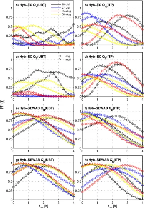
Fig. 8.Cross correlationR2(t )of simulated fluxes against flux reference shifted bytlagas multiples of 10 minutes for each of the four days simulated with the original and modyfied Hybrid. The maximum number of elements used in the calculation ofR2for each curve can be taken from Table 3.
into account the night-time, where fluxes and therefore ab-solute differences are smaller. The small improvement of RMSD ofQH andQHEC,EBC at ITP can be explained by the fact that the modified Hybrid follows the dynamics of EC, but flux estimates are larger and of the same magnitude as fluxes calculated by SEWAB. Mauder et al. (2006) have estimated the error or EC measurements to be 5 % or<10 W m2 for
QHand 15 % or<30 W m−2forQE. Additional uncertainty
Table 3. Root mean square deviation (RMSD) between the modelled quantities of the original and modified Hybrid and reference values. The reference quantities used are either measured by EC and corrected for energy balance closure (EC,EBC) or modelled with SEWAB for fluxes or taken from longwave outgoing radiation forT0. The values in parenthesis (N) correspond to the number of elements used for calculation of RMSD andR2(l=0)in Fig. 8.
RMSD
Site Date Run QE QH QE QH T0
EC,EBC [W m−2] SEWAB [W m−2] [◦C]
UBT
10 July
orig
318 117 (8) 94 74 (94) 4.3 (139)
27 July 97 58 (19) 60 59 (139) 4.5 (143)
5 August 168 139 (11) 90 64 (110) 4.3 (143)
6 August 159 84 (52) 87 71 (128) 3.7 (143)
ITP
10 July
orig
182 93 (25) 97 69 (143) 3.7 (143)
27 July 43 64 (72) 58 75 (143) 3.8 (143)
5 August 224 103 (64) 179 68 (143) 8.3 (143)
6 August 118 80 (52) 130 119 (143) 5.1 (143)
UBT
10 July
mod
214 43 (8) 51 36 (94) 2.3 (139)
27 July 79 44 (19) 32 28 (139) 2.9 (143)
5 August 93 62 (11) 36 26 (110) 3.4 (143)
6 August 78 57 (52) 39 32 (128) 3.2 (143)
ITP
10 July
mod
74 73 (25) 42 32 (143) 1.6 (143)
27 July 42 58 (72) 55 36 (143) 2.6 (143)
5 August 44 80 (64) 64 30 (143) 2.6 (143)
6 August 68 82 (52) 113 77 (143) 3.5 (143)
UBT all orig 170 92 (90) 83 67 (471) 4.2 (568)
mod 100 54 (90) 39 31 (471) 3.0 (568)
ITP all orig 152 84 (213) 125 86 (572) 5.6 (572)
mod 54 73 (213) 74 48 (572) 2.7 (572)
2006; Mauder et al., 2007). Therefore, additional research, such as high-resolution atmospheric modelling studies, need to be carried out in order to determine the contributions of
QH andQE to the “missing” energy. It should be noted
that all modelled fluxes and measurements have errors, so that there is no absolute way of knowing which method pro-duces the best flux estimates. The incorporation of surface fluxes into a regional circulation model may give some in-sight into whether modelled surface atmosphere interactions lead to realistic atmospheric flow patterns.
The large negative and potentially unreasonable night-time
QH-fluxes that are modelled for ITP on 6 August are owed to
a frozen soil and strong surface winds that lead to an overes-timation of the temperature gradient, delayed reaction of the surface model and resulted in a potential underestimation of modelled surface temperatures and thus surface fluxes.
5.2 Discussion of surface temperature
For surface temperature there is a notable decrease in RMSD for all cases. Additionally, the source of the error changes. In the original model the error inT0was mainly due to the
time-lag and a general underestimation of daytime maximum
surface temperatures. In the new model daytimeT0matches
a lot better with observations except for ITP 6 August, where evaporative cooling due to excessive evapotranspiration con-tributes to too small warming rates. In return, the cooling during the nighttime is overestimated. This may either be due to errors in soil moisture, surface emissivity (ǫ) or due to the surface temperature extrapolation function used in this work.
5.3 Soil moisture variation and evapotranspiration
if it were not restarted every day. This is caused by a very limited soil hydrology included in Hybrid. Hu et al. (2008) have estimated the summer evapotranspiration on a central Tibetan grassland site to be in the order of 4–6 mm d−1. An
experiment conducted within the framework of TiP has esti-mated bare soil evaporation and evapotranspiration of a very dry soil at Kema in 2010 (∼150 km northeast of Nam Co Lake) at 2 mm d−1rising to at least 6 mm d−1 and possibly more for a vegetatedKobresia pasture during an irrigation experiment (H. Coners – University of G¨ottingen, personal communication, 27 June 2011). Even though the soils are not directly comparable this suggests similar dynamics inQE
to the ITP site. One factor likely to play a role in the local water cycle that is not included is dew fall in the early morn-ing hours. Direct absorption of atmospheric moisture on bare soil (Agam (Ninari) and Berliner, 2004) and dew fall are of-ten considered a significant moisture input for semi-arid en-vironments (Agam and Berliner, 2006). Heavy dewfall in the vicinity of Nam Co Lake is frequently observed, but has, at least to our knowledge, never been quantified. This addi-tional source of water and the associated local recycling of water may account for a significant fraction of the missing water. In addition to this, the too simplistic representation of soil hydrology is very likely responsible for the remaining water deficit in the upper layer of the soil model.
5.4 Cross correlation of turbulent fluxes
A different way of looking at the model performance is cross correlation of the modelled surface fluxes against EC mea-surements and SEWAB (Fig. 8). These measures give an insight into the reasons for the delayed response of the sur-face model and the amount of flux-variance explained, but does not yield information whether the model and the ref-erence fluxes show a true one-to-one correlation. As with RMSD the quality of the analysis is limited by the number of data points that can be correlated, which is comparatively small for the energy balance corrected EC measurements at ITP and even smaller at UBT due to lake breeze influences (Fig. 8a–e). Hence, it is very difficult to interpret the cross correlations for EC. It is probably fair to say that there is a tendency for smaller time lags during the time series with higher number of elements, notably UBT 6 August and all days of ITP and that the total explained variances are at the same level of determination, when comparing the maximum
R2(j ). A notable exception is ITP 5 August.
For the comparison with SEWAB (Fig. 8f–h), it becomes notable that for many cases the maximumR2(j )of the modi-fied Hybrid approachR2 →1 and that their maxima are usu-ally found at lags of 10–30 min (j=1−3). Solar radiation rapidly modifies the skin temperature that is governing tur-bulent fluxes. As SEWAB has an instantaneous surface tem-perature solver for each model time step, one would expect a direct response of SEWAB to changes in solar radiation. This may even be faster than in reality, especially forQEflux that
is not only dependent on the actual skin temperature, but also on the vegetation’s response. Including negative values ofj
into Fig. 8 would show a gradual decrease of correlations with decreasingj, showing that the flux dynamics of Hybrid never precede EC measurements or SEWAB.
5.5 Natural variability of fluxes
Atmospheric quantities and turbulent surface fluxes have a large natural variability that is difficult to measure or to model. The EC approach is dependent on averaging proce-dures and most standard measurements will yield mean val-ues. In order to use high-frequency measurements for flux estimation, less common techniques such as conditional sam-pling or wavelet-spectra have to be used. Even if models are capable of reproducing variability on realistic scales it is difficult to supply forcing data with similar resolution. The forcing data used in this study, sampled and averaged 10 or 30 min means, are used for SEWAB. Running Hybrid at time steps comparable to a high-resolution mesoscale model re-quires interpolation of the forcing data and therefore poten-tially causes a smoothing of the model’s response compared to the actual weather forcing as it would be provided by a coupled model. As surface models share a similar approach to the parameterisation of surface fluxes and close the surface energy balance locally, SEWAB and Hybrid fluxes are more similar to each other than they are to field measurements.
6 Conclusions
The accurate generation of surface fluxes is a necessary pre-requisite for studies of surface-atmosphere interactions and local to mesoscale circulations. In order to gain a better pro-cess understanding of the interaction between atmospheric circulation, clouds, radiation and surface fluxes, the gener-ated diurnal flux cycles have to be of realistic magnitude and without temporal shift. The original two-layer surface model without a specific formulation forT0produced both a
consid-erable time lag and failed to capture the full diurnal dynamics due to its unresponsiveness.
We have demonstrated that the introduction of an extrapo-lated surface temperature enables even a quite simplistic soil model to realistically simulate skin temperatures and thus to generate more realistic surface fluxes. The delay of fluxes during the daily cycle was greatly reduced, making the model usable for diurnal process studies. The total magnitude of fluxes is also much improved, when few and computationally cheap additional physically based processes are introduced. Comparing SEWAB with Hybrid, the RMSD for both fluxes and surface temperature is decreased by generally 40–60 %. The improvement in quality was somewhat more varied in comparison to EC measurements, as comparison of models and measurements is not straight forward. The improved
the flux time series have been greatly reduced and the over-all correlations are high. As with any natural system it is impossible to obtain complete data sets that capture the full amount of natural variability. However, the modified model has been tested for a larger spectrum of environmental condi-tions on the TP and produced reasonable results for both dry and moist conditions.
We have shown that a rather simple soil surface model can efficiently calculate turbulent fluxes at a high temporal reso-lution when driven by realistic atmospheric conditions. Nev-ertheless, it is quite clear that such an approach with extrapo-lated surface temperature needs careful model initialisation. The initial soil heat contents and therefore knowledge of soil temperature profiles is necessary. Due to the fact that the surface temperature in this study is a purely diagnostic quan-tity, there may still be some limitations such as a delayed or smoothed response to atmospheric forcing on very short timescales, such as the feedback between passing boundary-layer clouds and the surface fluxes. The influence of sur-face fluxes and their dynamics to regional circulation will be investigated in a future study.
Acknowledgements. This research was funded by the German Research Foundation (DFG) Priority Programme 1372 “Tibetan Plateau: Formation, Climate, Ecosystems” as part of the Atmo-sphere – Ecology – Glaciology Cluster (TiP-AEG). ITP data was provided through CEOP-AEGIS, which is a EU-FP7 Collaborative Project/ Small or medium-scale focused research project – Specific International Co-operation Action coordinated by the University of Strasbourg, France under the call ENV.2007.4.1.4.2: “Improving observing systems for water resource management.” The authors would like to thank everyone who has contributed to the collection of field data in one of the world’s most remote regions. ADF acknowledges support from the European Community’s Seventh Framework Programme (FP7/2007-2013) under grant agreement no. 238366. AH acknowledges funding by the Fonds National de la Recherche (FNR-Luxembourg), under the grant BFR07-089 and support by the Cambridge European Trust (CET-UK).
Edited by: C. de Michele
References
Agam (Ninari), N. and Berliner, P. R.: Diurnal Water Content Changes in the Bare soil of a coastal desert, J. Hydrometeorol., 5, 922–933, doi:10.1175/1525-7541(2004)005<0922:DWCCIT>2.0.CO;2, 2004.
Agam, N. and Berliner, P. R.: Dew formation and water vapor ad-sorption in semi-arid environments – A review, J. Arid Environ., 65, 572–590, doi:10.1016/j.jaridenv.2005.09.004, 2006. Aubinet, M., Grelle, A., Ibrom, A., Rannik, U., Moncrieff, J.,
Fo-ken, T., Kowalski, A., Martin, P., Berbigier, P., Bernhofer, C., Clement, R., Elbers, J., Granier, A., Gr¨unwald, T., Morgen-stern, K., Pilegaard, K., Rebmann, C., Snijders, W., Valentini, R., Vesala, T., Fitter, A., and Raffaelli, D.: Estimates of the an-nual net carbon and water exchange of forests: The EUROFLUX
Methodology, Adv. Ecol. Res., 30, 113–175, doi:10.1016/S0065-2504(08)60018-5, 1999.
Biermann, T., Babel, W., Olesch, J., and Foken, T.: Mesoscale cir-culations and energy and gas exchange over the Tibetan Plateau – Documentation of the micrometeorological experiment, Nam Tso, Tibet – 25 June–8 August 2009, Arbeitsergebnisse 41, Uni-versity of Bayreuth, ISSN 1614-8616, Bayreuth, 2009.
Blackadar, A.: High resolution models of the planetary boundary layer, in: Advances in Environmental Science and Engineering, edited by: Pfafflin, J. and Ziegler, E., Vol. 1, 50–85, Gordon and Breach, New York, 1979.
Camillo, P. J. and Gurney, R. J.: A resistance parameter for bare-soil evaporation models, Soil Sci., 141, 95–105, 1986.
Cong, Z., Kang, S., Smirnov, A., and Holben, B.: Aerosol optical properties at Nam Co, a remote site in central Tibetan Plateau, Atmos. Res., 92, 42–48, doi:10.1016/j.atmosres.2008.08.005, 2009.
Cui, X., Langmann, B., and Graf, H.: Summer monsoonal rainfall simulation on the Tibetan Plateau with a regional climate model using a one-way double-nesting system, SOLA, 3, 49–52, 2007. Deardorff, J. W.: Dependence of air-sea transfer coefficients on bulk
stability, J. Geoph. Res., 73, 2549–2557, 1968.
Fairall, C. W., Bradley, E. F., Godfrey, J. S., Wick, G. A., Edson, J. B., and Young, G. S.: Cool-skin and warm-layer effects on sea surface temperature, J. Geophys. Res., 101, 1295–1308, 1996a. Fairall, C. W., Bradley, E. F., Rogers, D. P., Edson, J. B., and
Young, G. S.: Bulk parameterization of air-sea fluxes for Tropi-cal Ocean-Global Atmosphere Coupled-Ocean Atmosphere Re-sponse Experiment, J. Geophy. Res., 101, 3747–3764, 1996b. Foken, T.: The parameterisation of the energy exchange across
the air-sea interface, Dynam. Atmos. Ocean, 8, 297–305, doi:10.1016/0377-0265(84)90014-9, 1984.
Foken, T.: The energy balance closure problem: An overview, Ecol. Appl., 18, 1351–1367, 2008.
Foken, T., G¨ockede, M., Mauder, M., Mahrt, L., Amiro, B., and Munger, J.: Post field data quality control, in: Handbook of Micrometeorology: A guide for surface flux measurements and analysis, edited by: Lee, X., Massman, W., and Law, B., 181– 208, Kluwer, Dordrecht, 2004.
Foken, T., Aubinet, M., Finnigan, J. J., Leclerc, M. Y., Mauder, M., and Paw U, K. T.: Results Of A Panel Discussion About The En-ergy Balance Closure Correction For Trace Gases, B. Am. Me-teorol. Soc., 92, ES13–ES18, doi:10.1175/2011BAMS3130.1, 2011.
Freedman, J. M., Fitzjarrald, D. R., Moore, K. E., and Sakai, R. K.: Boundary layer clouds and vegetation-atmosphere feedbacks, J. Climate, 14, 180–197, doi:10.1175/1520-0442(2001)013<0180:BLCAVA>2.0.CO;2, 2001.
Friend, A. D.: Terrestrial plant production and climate change, J. Exp. Bot., 61, 1293–1309, doi:10.1093/jxb/erq019, 2010. Friend, A. D. and Kiang, N. Y.: Land surface model development
for the GISS GCM: effects of improved canopy physiology on simulated climate, J. Climate, 18, 2883–2902, 2005.
Friend, A. D., Stevens, A. K., Knox, R. G., and Cannell, M. G. R.: A process-based, terrestrial biosphere model of ecosystem dy-namics (Hybrid v3.0), Ecol. Model., 95, 249–287, 1997. Hansen, J., Russell, G., Rind, D., Stone, P., Lacis, A., Lebedeff,
111, 609–662, 1983.
Herzog, M., Graf, H., Textor, C., and Oberhuber, J. M.: The ef-fect of phase changes of water on the development of volcanic plumes, J. Volcanol. Geoth. Res., 87, 55–74, doi:10.1016/S0377-0273(98)00100-0, 1998.
Hu, Z., Yu, G., Fu, Y., Sun, X., Li, Y., Shi, P., Wang, Y., and Zheng, Z.: Effects of vegetation control on ecosystem water use efficiency within and among four grassland ecosystems in China, Glob. Change Biol., 14, 1609–1619, doi:10.1111/j.1365-2486.2008.01582.x, 2008.
Hu, Z., Yu, G., Zhou, Y., Sun, X., Li, Y., Shi, P., Wang, Y., Song, X., Zheng, Z., Zhang, L., and Li, S.: Partitioning of evapotranspira-tion and its controls in four grassland ecosystems: Applicaevapotranspira-tion of a two-source model, Agric. For. Meteorol., 149, 1410–1420, doi:10.1016/j.agrformet.2009.03.014, 2009.
Kanda, M., Inagaki, A., Letzel, M. O., Raasch, S., and Watan-abe, T.: LES Study of the energy imbalance problem with eddy covariance fluxes, Bound.-Lay. Meteorol., 110, 381–404, doi:10.1023/B:BOUN.0000007225.45548.7a, 2004.
Keil, A., Berking, J., M¨ugler, I., Sch¨utt, B., Schwalb, A., and Steeb, P.: Hydrological and geomorphological basin and catchment characteristics of Lake Nam Co, South-Central Tibet, Quart. Int., 218, 118–130, 2010.
Kracher, D., Mengelkamp, H., and Foken, T.: The residual of the energy balance closure and its influence on the re-sults of three SVAT models, Meteorologische Z., 18, 647–661, doi:10.1127/0941-2948/2009/0412, 2009.
Kuwagata, T., Kondo, J., and Sumioka, M.: Thermal effect of the sea breeze on the structure of the boundary layer and the heat budget over land, Bound.-Lay. Meteorol., 67, 119–144, doi:10.1007/BF00705510, 1994.
Li, M., Ma, Y., Hu, Z., Ishikawa, H., and Oku, Y.: Snow distri-bution over the Namco lake area of the Tibetan Plateau, Hy-drol. Earth Syst. Sci., 13, 2023–2030, doi:10.5194/hess-13-2023-2009, 2009.
Lohou, F. and Patton, E. G.: Land-surface response to shal-low cumulus, EGU General Assembly, Vienna, Austria, 3– 8 April 2011, EGU2011-10280-1, 2011.
Ma, Y., Wang, Y., Wu, R., Hu, Z., Yang, K., Li, M., Ma, W., Zhong, L., Sun, F., Chen, X., Zhu, Z., Wang, S., and Ishikawa, H.: Re-cent advances on the study of atmosphere-land interaction ob-servations on the Tibetan Plateau, Hydrol. Earth Syst. Sci., 13, 1103–1111, doi:10.5194/hess-13-1103-2009, 2009.
Mauder, M. and Foken, T.: Documentation and instruction man-ual of the eddy covariance software package TK3, Arbeitsergeb-nisse 46, University of Bayreuth, ISSN 1614-8916, Bayreuth, 2011.
Mauder, M., Oncley, S. P., Vogt, R., Weidinger, T., Ribeiro, L., Bernhofer, C., Foken, T., Kohsiek, W., Bruin, H. A. R., and Liu, H.: The energy balance experiment EBEX-2000. Part II: Intercomparison of eddy-covariance sensors and post-field data processing methods, Bound.-Lay. Meteorol., 123, 29–54, doi:10.1007/s10546-006-9139-4, 2006.
Mauder, M., Desjardins, R. L., and MacPherson, I.: Scale anal-ysis of airborne flux measurements over heterogeneous ter-rain in a boreal ecosystem, J. Geophys. Res., 112, D13112, doi:10.1029/2006JD008133, 2007.
Mauder, M., Foken, T., Clement, R., Elbers, J. A., Eugster, W., Gr¨unwald, T., Heusinkveld, B., and Kolle, O.: Quality
control of CarboEurope flux data – Part 2: Inter-comparison of eddy-covariance software, Biogeosciences, 5, 451–462, doi:10.5194/bg-5-451-2008, 2008.
Mengelkamp, H., Warrach, K., and Raschke, E.: SEWAB – a pa-rameterization of the surface energy and water balance for atmo-spheric and hydrologic models, Adv. Wat. Resour., 23, 165–175, doi:10.1016/S0309-1708(99)00020-2, 1999.
Metzger, S., Ma, Y., Markkanen, T., G¨ockede, M., Li, M., and Fo-ken, T.: Quality assessment of Tibetan Plateau Eddy covariance measurements utilizing footprint modeling, Adv. Earth Sci., 21, 1260–1267, 2006.
Miehe, G., Miehe, S., Bach, K., N¨olling, J., Hanspach, J., Reuden-bach, C., Kaiser, K., Wesche, K., Mosbrugger, V., Yang, Y., and Ma, Y.: Plant communities of central Tibetan pastures in the Alpine Steppe/Kobresia pygmaea ecotone, J. Arid Environ., 75, 711–723, doi:10.1016/j.jaridenv.2011.03.001, 2011.
Oberhuber, J. M., Herzog, M., Graf, H., and Schwanke, K.: Vol-canic plume simulation on large scales, J. Volcanol. Geoth. Res., 87, 29–53, doi:10.1016/S0377-0273(98)00099-7, 1998. Panin, G. N., Tetzlaff, G., and Raabe, A.: Inhomogeneity of the
land surface and problems in the parameterization of surface fluxes in natural conditions, Theor. Appl. Climatol., 60, 163–178, doi:10.1007/s007040050041, 1998.
Panin, G. N., Nasonov, A. E., and Foken, T.: Evaporation and heat exchange of a body of water with the atmosphere in a shallow zone, Izvestiya, Atmos. Ocean. Phys., 42, 337–352, doi:10.1134/S0001433806030078, 2006.
Ruppert, J., Thomas, C., and Foken, T.: Scalar similarity for relaxed eddy accumulation methods, Bound.-Lay. Meteorol., 120, 39– 63, doi:10.1007/s10546-005-9043-3, 2006.
Sellers, P. J., Mintz, Y., Sud, Y. C., and Dalcher, A.: A Simple Bio-sphere Model (SIB) for use within general circulation models, J. Atmos. Sci., 43, 505–531, 1986.
Su, Z., Wen, J., Dente, L., van der Velde, R., Wang, L., Ma, Y., Yang, K., and Hu, Z.: The Tibetan Plateau observatory of plateau scale soil moisture and soil temperature (Tibet-Obs) for quanti-fying uncertainties in coarse resolution satellite and model prod-ucts, Hydrol. Earth Syst. Sci., 15, 2303–2316, doi:10.5194/hess-15-2303-2011, 2011.
Twine, T. E., Kustas, W. P., Norman, J. M., Cook, D. R., Houser, P. R., Meyers, T. P., Prueger, J. H., Starks, P. J., and Wesely, M. L.: Correcting eddy-covariance flux underes-timates over a grassland, Agric. For. Meteorol., 103, 279–300, doi:10.1016/S0168-1923(00)00123-4, 2000.
van Heerwaarden, C. C., de Arellano, J. V., Moene, A. F., and Holt-slag, A. A. M.: Interactions between dry-air entrainment, surface evaporation and convective boundary-layer development, Q. J. Roy. Meteorol. Soc., 135, 1277–1291, doi:10.1002/qj.431, 2009. Xue, Y., Zeng, F. J., and Schlosser, C. A.: SSiB and its sensi-tivity to soil properties – a case study using HAPEX-Mobilhy data, Glob. Planet. Change, 13, 183–194, doi:10.1016/0921-8181(95)00045-3, 1996.
Yang, K., Koike, T., and Yang, D.: Surface flux parameterization in the Tibetan Plateau, Bound.-Lay. Meteorol., 106, 245–262, doi:10.1023/A:1021152407334, 2003.
Yee, S. Y. K.: The force-restore method revisited, Bound.-Lay. Me-teorol., 43, 85–90, doi:10.1007/BF00153970, 1988.
You, Q. L., Kang, S. C., Li, C. L., Li, M. S., and Liu, J. S.: Fea-tures of meteorological parameters at Nam Co station, Tibetan Plateau, in: Annual Report of Nam Co Monitoring and Research Station for Multisphere Interactions, edited by: Nam Co Mon-itoring and Research Station for Multisphere Interaction, 1–8, Chinese Academy of Sciences, Beijing, 2006 (in Chinese with English abstract).
![Fig. 1. Landcover map of study area: the black cross indicates the station identified as UBT, close to the small lake with denser surface cover [grass (+)], the red cross shows the station location ITP with sparse surface cover [grass (-)].](https://thumb-eu.123doks.com/thumbv2/123dok_br/16284833.184924/2.892.463.819.96.366/landcover-indicates-station-identified-surface-station-location-surface.webp)
![Fig. 2. Forcing data measured at UBT used for model runs: (a) downward shortwave radiation (SW [W m −2 ]); b) downward longwave radiation (LW [W m −2 ]); (c) air temperature (T [ ◦ C]); (d) water vapour mixing ratio (q [g kg −1 ]); (e) wind speed (U [m s −](https://thumb-eu.123doks.com/thumbv2/123dok_br/16284833.184924/3.892.148.745.92.382/forcing-measured-downward-shortwave-radiation-longwave-radiation-temperature.webp)