www.atmos-chem-phys.net/16/5315/2016/ doi:10.5194/acp-16-5315-2016
© Author(s) 2016. CC Attribution 3.0 License.
Comparison of eddy covariance and modified Bowen ratio methods
for measuring gas fluxes and implications for
measuring fluxes of persistent organic pollutants
Damien Johann Bolinius1, Annika Jahnke1,2, and Matthew MacLeod1
1Department of Environmental Science and Analytical Chemistry (ACES), Stockholm University, Svante Arrhenius väg 8, 114 18, Stockholm, Sweden
2Department Cell Toxicology, Helmholtz Centre for Environmental Research (UFZ), Permoserstr. 15, 04318 Leipzig, Germany
Correspondence to:Damien Johann Bolinius ([email protected])
Received: 7 September 2015 – Published in Atmos. Chem. Phys. Discuss.: 20 November 2015 Revised: 15 April 2016 – Accepted: 18 April 2016 – Published: 28 April 2016
Abstract.Semi-volatile persistent organic pollutants (POPs) cycle between the atmosphere and terrestrial surfaces; how-ever measuring fluxes of POPs between the atmosphere and other media is challenging. Sampling times of hours to days are required to accurately measure trace concentrations of POPs in the atmosphere, which rules out the use of eddy co-variance techniques that are used to measure gas fluxes of major air pollutants. An alternative, the modified Bowen ra-tio (MBR) method, has been used instead. In this study we used data from FLUXNET for CO2and water vapor (H2O) to compare fluxes measured by eddy covariance to fluxes measured with the MBR method using vertical concentra-tion gradients in air derived from averaged data that simulate the long sampling times typically required to measure POPs. When concentration gradients are strong and fluxes are unidi-rectional, the MBR method and the eddy covariance method agree within a factor of 3 for CO2, and within a factor of 10 for H2O. To remain within the range of applicability of the MBR method, field studies should be carried out under conditions such that the direction of net flux does not change during the sampling period. If that condition is met, then the performance of the MBR method is neither strongly affected by the length of sample duration nor the use of a fixed value for the transfer coefficient.
1 Introduction
Despite the more than decade-old global ban on the produc-tion and use of persistent organic pollutants (POPs) such as polychlorinated biphenyls (PCBs), hexachlorobenzene and several organochlorine pesticides, these chemicals are still present in the environment and continue to raise concerns due to their persistence, bioaccumulation, toxicity and poten-tial for long-range atmospheric transport (The Secretariat of the Stockholm Convention, 2010). As the production and use of POPs continues to decline, large cities, old stocks and re-volatilization from soil are expected to become more impor-tant sources to the atmosphere (Nizzetto et al., 2010). Study-ing the sources and fate of organic pollutants in the environ-ment is an important prerequisite to exposure and risk assess-ment; and environmental fate models that calculate fluxes of pollutants between air, water, soil, vegetation and other me-dia have proven to be valuable tools in this respect (McKone and MacLeod, 2003). Measurements of fluxes of POPs em-anating from source areas and between the atmosphere and other environmental media are needed to parameterize and evaluate the chemical fate models that are used as scientific support for international conventions on POPs (Gusev et al., 2012).
velocity, using data from very fast measurements (e.g. 5– 10 Hz). This approach works well for compounds such as CO2, methane, ozone and more recently also for mercury (Pierce et al., 2015), since concentrations can be measured at a high temporal resolution. However, it cannot be applied di-rectly when studying trace-level organic micropollutants that require sampling times of a minimum of several hours when using active high-volume sampling, or even several weeks when using passive samplers (Hung et al., 2013).
One way to estimate chemical fluxes from measurements based on sampling times of hours to days is to use the modified Bowen ratio (MBR) method (Businger, 1986). The MBR method is based on the assumption that turbulent atmo-spheric transport occurs indiscriminately for chemicals, heat and other scalar quantities that can be described entirely by their magnitude without reference to direction. It can be used to measure the flux of a chemical pollutant (x) from measure-ments of its concentration at two heights and the measured transfer coefficient of another scalar such as heat (y) over the same height interval (Meyers et al., 1996, Eq. 1):
Fx= −Ky·1Cx
1Z , (1)
where Fx (ng m−2h−1) is the flux of chemical x, Ky (m2h−1)is the measured eddy diffusion coefficient for scalar
y over the height interval1Z (m) and1Cx(ng m−3)is the measured concentration gradient ofx over the height inter-val. The negative sign on the right-hand side of the equation enforces the convention that downward fluxes have a nega-tive sign, and upward fluxes a posinega-tive sign.
Among other applications, the MBR method has been used to measure volatilization fluxes of pesticides applied to agricultural fields (Majewski, 1999), to estimate PCB fluxes from Lake Superior to the overlying air (Rowe and Per-linger, 2012) and fluxes of polycyclic aromatic hydrocarbons (PAHs) above a forest canopy in Canada (Choi et al., 2008). In the study of Choi et al. (2008) air was sampled for 24 h ev-ery 3 days at different heights for a period of 1 month while leaves in the forest canopy were developing. The samples were analyzed for PAHs and the data were combined with the eddy diffusivity of heat (Kheat)determined from eddy covari-ance measurements from the FLUXNET network to estimate vertical PAH fluxes using the MBR method.
Our goal in this study was to test the limits of applica-bility of the MBR method and to evaluate its accuracy rel-ative to the “standard” EC technique. We used data from the FLUXNET network to calculate fluxes of CO2and wa-ter vapor (H2O) with the MBR method under different sam-pling duration scenarios and different assumptions about data availability for the eddy diffusion coefficientKy. Thus, we took advantage of the high-frequency measurement data for CO2 and H2O, and used them as proxies for organic mi-cropollutants in order to analyze the performance of the MBR method compared to the EC method. By averaging the FLUXNET data over periods that ranged from 1 h to 1 week,
we simulated sampling times that are typically required to measure POPs and other organic micropollutants in air. Our approach is similar to the one used by Majewski (1999), who simulated 24 h sampling periods from higher frequency data to characterize the potential for long sampling times to intro-duce error to the aerodynamic profiling method.
2 Methods 2.1 Data sets
All data used in this study can be accessed freely via the FLUXNET home page (http://fluxnet.ornl.gov/). A figure showing the flux tower and associated instruments can be found in the Supplement Fig. S1. The data set used in this study contains eddy flux parameters and micrometeorolog-ical measurements for the year 2009 taken at the Borden mixed deciduous forest site in Ontario, Canada (FLUXNET site code: CA-Cbo). A list of all parameters is given in Supplement Table S1. We selected measurements taken at heights of 33.3 and 40.7 m. Air sampling in the study by Choi et al. (2008) was conducted at the same site in 2003 at heights of 29.1 and 44.4 m.
Prior to any calculations, we filtered the data to remove about 25 % of the observations that were flagged as unreli-able for CO2or H2O. Details on the criteria for the flags can be found on the FLUXNET home page. Common reasons for flagging are instrument malfunctions, calibration prob-lems and outliers. All flagged data were filtered out simul-taneously, such that our analysis only includes data points collected at times when data were not flagged for either CO2 or H2O.
On inspection of the distribution of the CO2and H2O con-centration gradients, it was apparent that a few outliers that had not been flagged could significantly alter the average gra-dient when pooling the data to simulate long sampling times. These outliers in some cases led to net flux estimations based on the MBR method that were in the opposite direction com-pared to the EC method. To exclude such outliers and reduce the influence of extreme values of measured parameters, the highest and lowest 2.5 % of values of the CO2gradient and the H2O gradient were removed from the data set prior to further calculations.
2.2 Modified Bowen ratio
measured at 33 m height (1005.7 J kg−1K−1). SpuriousKheat values less than or equal to zero were removed from the data set as these would indicate a heat flux against the measured temperature gradient.
W′T′= Q
Cp·σair
(2)
Kheat (m2s−1)was then calculated based on temperatures measured at 40.7 and 33.3 m according to Eq. (3).
Kheat= −W′T′(40.7−33.3)
(T40.7−T33.3)
(3) Finally, vertical turbulent fluxes of CO2and H2O were cal-culated using the MBR method and measured concentrations at 33 and 41.5 m averaged over different time intervals se-lected to represent sampling times typical for organic mi-cropollutants, as described below. Fluxes calculated with the MBR method were compared with those measured by the EC method available from the FLUXNET data set.
2.3 Data analysis
To simulate sampling times typical for organic micropollu-tants, concentrations of CO2and H2O reported as 30 min av-erages in the database were pooled and averaged over periods of 1, 2, 4, 8 and 24 h, 3 days (72 h) and 1 week (168 h). Fluxes during four 2-month periods selected to represent each of the four seasons were then calculated from median values of these pooled data points during the entire period. Thus for ex-ample, fluxes calculated from 1 h simulated sampling times are based on the median of average vertical concentration gradients in 1 h pools measured at the same time each day over the entire 2 month period (see Fig. S2 for a visual rep-resentation). Medians were used instead of geometric means because of the presence of negative flux values. January and February represented winter, April and May spring, July and August summer and October and November fall.
We tested two approaches to specify Kheat in the MBR method calculations. In the first approach, hourly average
Kheat values were calculated from 30 min averages of tem-perature measurements reported in the database. In the sec-ond approach, a geometric mean ofKheatwas calculated for all time points across the entire period corresponding to the simulated sampling time. The first approach takes advantage of the availability of high temporal resolution information aboutKheatat the FLUXNET site, but the second approach is likely to be common when applying the MBR since high-frequency meteorological data are not always available.
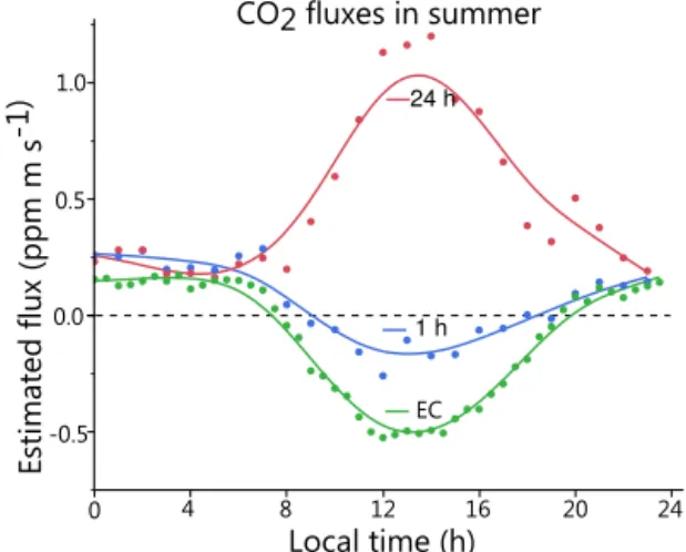
The direction of flux for CO2can change on a diurnal ba-sis (see Figs. 1 and S3). During the day, the flux of CO2is often negative (i.e., downward) due to photosynthesis, while during the night, plant respiration produces CO2and fluxes are positive (i.e. to the atmosphere). In addition, atmospheric conditions during the night are typically much more stable
than during the day, resulting in a lack of large turbulent ed-dies and a higher contribution of additional transport mech-anisms, such as horizontal advection, to the total flux. The result is that fluxes measured using EC during the night are often underestimated (Aubinet, 2008).
To understand the impact of changing directions of flux and to investigate potential underestimation of flux at night, fluxes during the day and during the night calculated with the MBR method were evaluated against EC measurements separately. Nighttime data were set to cover from 21:00 to 05:00 local time across all seasons, and daytime data were set from 09:00 to 17:00 local time. The nighttime/daytime di-visions were selected based on the shortest interval between sunrise and sunset at the site. The 8 h periods representing day and night allowed us to construct 24 h, 3 day and 1 week sampling periods by averaging a whole number of 8 h pe-riods taken at the same time of day over multiple days. In addition to the nighttime/daytime split data, we also exam-ined the performance of the MBR method relative to the EC method when using continuous data that ignored day/night differences.
3 Results
3.1 Kheatand concentration gradients
Our calculatedKheat values (Fig. 1) are in good agreement with values for the same site during the same time of year in 2003 (Choi et al., 2008, shown in Fig. S4). Values are close to 0 during the night and in the range of 0.0026 to 35.8 m2s−1 during the day over the summer period, with 95 % of the val-ues between 0.029 and 22.11 m2s−1.
The fluxes calculated with the MBR method are propor-tional to the product ofKheatand the concentration gradient of either CO2 or H2O (Eq. 1). The raw data at 30 min time resolution that were pooled and used to calculate the fluxes with the MBR method are visualized in Fig. 1.
3.2 Performance of the MBR method on continuous time series
Figure 1.Half-hourly averages ofKheatand the concentration gradients of CO2and H2O across the different seasons (concentration at 40.7 m – concentration at 33.3 m). The dotted line indicates 0 in all plots; the grey areas indicate the 8 h periods representing day and night.
CO28fluxes8in8summer
E
st
ima
te
d
8f
lu
x8
(p
p
m8
m8
s-1)
Local8time8(h) 1.0
0.5
0.0
-0.5
0 4 8 12 16 20 24
24 h
1 h
EC
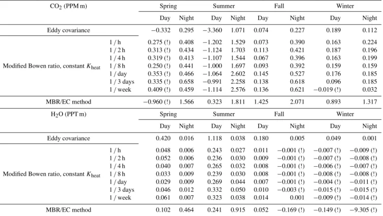
Figure 2. A comparison of measured fluxes using the modified Bowen ratio (MBR) method (1 and 24 h pooled data using hourly Kheat values) with the eddy covariance (EC) measurements. The simulated 24 h sampling time includes a change in the direction of the CO2 flux, which results in a measured flux with the MBR method that has the wrong direction and magnitude.
3.3 Performance of the MBR method with hourly resolved and fixed values ofKheat
The use of either hourly resolved data for Kheat or a fixed value did not significantly affect the MBR method. A student
ttest comparing the similarity of the two data sets resulted in aP value below 0.0001.
Results using a fixed value forKheatare shown in Table 1; those using hourly resolved data forKheatare given in Sup-plement Table S2.
3.4 Performance of the MBR method on day/night split data
Table 1. Cumulative fluxes for 8 h periods representing day and night across the 2 month periods representing spring, summer, fall and winter. Fluxes measured by the MBR method that are in the opposite direction to those measured by the EC method are marked with “(!)”. Positive fluxes are defined as fluxes moving upwards from the canopy. The ratio of MBR results over EC results is based on the geometric mean of the MBR results divided by the EC result. The MBR fluxes for the 1 week sampling period were left out in the calculation of the geometric mean during the day in winter for CO2and during the night in fall for H2O. This table shows fluxes calculated with a fixed value forKheat.
CO2(PPM m) Spring Summer Fall Winter
Day Night Day Night Day Night Day Night
Eddy covariance −0.332 0.295 −3.360 1.071 0.074 0.227 0.189 0.112
Modified Bowen ratio, constantKheat
1/h 0.275 (!) 0.408 −1.202 1.529 0.073 0.390 0.163 0.224
1/2 h 0.313 (!) 0.434 −1.124 1.703 0.113 0.421 0.187 0.196
1/4 h 0.319 (!) 0.413 −1.107 1.544 0.067 0.396 0.163 0.199
1/8 h 0.250 (!) 0.441 −1.000 1.697 0.093 0.392 0.159 0.159
1/day 0.353 (!) 0.466 −1.064 2.602 0.145 0.527 0.176 0.185
1/3 days 0.335 (!) 0.658 −0.991 2.258 0.138 0.618 0.096 0.185
1/week 0.409 (!) 0.459 −1.114 2.576 0.136 0.621 −0.019 (!) 0.032
MBR/EC method −0.960 (!) 1.566 0.323 1.811 1.425 2.071 0.893 1.317
H2O (PPT m) Spring Summer Fall Winter
Day Night Day Night Day Night Day Night
Eddy covariance 0.420 0.016 1.118 0.038 0.180 0.005 0.049 0.001
Modified Bowen ratio, constantKheat
1/h 0.048 0.006 0.243 0.027 0.011 −0.001 (!) −0.007 (!) −0.009 (!)
1/2 h 0.052 0.006 0.236 0.030 0.009 −0.001 (!) −0.007 (!) −0.008 (!)
1/4 h 0.040 0.007 0.265 0.032 0.008 −0.001 (!) −0.006 (!) −0.007 (!)
1/8 h 0.033 0.009 0.239 0.030 0.008 −0.001 (!) −0.008 (!) −0.008 (!)
1/day 0.029 0.009 0.269 0.044 0.007 −0.001 (!) −0.004 (!) −0.011 (!)
1/3 days 0.046 0.012 0.332 0.050 0.010 −0.003 (!) −0.015 (!) −0.015 (!)
1/week 0.061 0.007 0.323 0.038 0.014 0.001 −0.009 (!) −0.014 (!)
MBR/EC method 0.102 0.464 0.241 0.915 0.052 −0.169 (!) −0.149 (!) −9.305 (!)
fluxes with the opposite sign compared to the EC method during the spring and for the 1 week duration simulated sam-pling scenario in the winter (values marked with “(!)” in Ta-ble 1). In those cases where the direction of flux calculated with the MBR does not agree with the EC method, the dis-agreement is attributable to the median value of1CO2 (be-tween 41.5 and 33 m) selected to represent the sampling pe-riod, with a sign that implies a flux in the opposite direction of the flux measured with the EC method.
In cases where the direction of daytime flux measured us-ing the MBR method agreed with the EC method, the ratio of the two fluxes ranged from 0.32 to 1.4, implying that the two methods differed by factors that range from 1.4 to 3.0 and that the MBR method may either underestimate or over-estimate fluxes relative to the EC method.
For H2O, the fluxes measured with the MBR method are in the same direction as those measured by the EC method during spring, summer and during the day in the fall. When the two methods agree about the direction of flux, the ratio of fluxes measured by the MBR method to the EC method is between 0.9 and 0.052, implying differences between the methods by factors of 1.1 to 20, and that fluxes of H2O are underestimated if the MBR method is applied as compared
to the EC method. Fluxes measured during the winter sea-son with the MBR method are negative (i.e., from the atmo-sphere to the surface), while the EC method indicates fluxes are positive (i.e., from the surface to the atmosphere). Fluxes measured by both methods during the night in the fall are small, with an upward flux measured using the EC method and downward fluxes measured by the MBR method in all cases except the longest 1 week simulated sampling period.
In general, the fluxes measured using the two different methods are in better agreement for CO2than for H2O (Ta-ble 1). It is interesting to note that the MBR method gener-ally overestimates the flux of CO2relative to the EC method, while it underestimates fluxes of H2O in most cases.
4 Discussion
con-centration gradient for the compound of interest. The error arises because the average values ofKheatare dominated by high values that occur during the day, while average values of1CO2are dominated by extreme values that occur at night (see especially the summer season for CO2in Fig. 1 and data for CO2in the summer visualized in Fig. S5).
The CO2 fluxes determined using the MBR method dur-ing the daytime for the sprdur-ing season and when simulatdur-ing a sampling time of 1 week during daytime for the winter were in the opposite direction relative to the fluxes determined us-ing the EC method. Durus-ing sprus-ing this could be caused by a reversal of the direction of flux due to the development of leaves and the start of photosynthesis taking place halfway through the season, which would produce a shift from a con-tinuous net flux of CO2 out of the canopy to a diel cycle of CO2 uptake and release. Furthermore, it is possible that the simulated 1 week sampling duration during daytime in the winter might have encompassed periods when the net di-rection of flux of CO2changed, due to the movement of air masses with variable CO2concentrations across the region. Thus, all of the cases of disagreement between the MBR method and the EC method about the direction of flux of CO2 that are shown in Table 2 might be attributable to ap-plying the MBR method using simulated sampling times that encompass a change of direction of the net flux.
In general, the duration of simulated sampling does not have a strong influence on the fluxes measured with the MBR method. Exceptions are the longest simulated sampling times during the daytime in winter for CO2and during nighttime in the fall for H2O. We simulated sampling times of 24 h, 3 days and 1 week by combining data that were measured over non-consecutive 8 h periods during 2 month time win-dows selected to represent the four seasons. For the 3 day and 1 week simulated sampling times there are just three to four data points per season, depending on the data availabil-ity, which may introduce higher uncertainty in the median value used in our MBR method calculations compared to the shorter simulated sampling times.
For H2O, which nearly always has a net flux moving up-wards from the canopy during both the day and the night, pooling of the data over longer time intervals and application of the MBR method also led to estimations of the direction of flux that were opposite to the EC method in the winter and fall seasons. In winter, fluxes of H2O measured by the EC method were small and moving upwards, while those calculated with the MBR method were small and moving downwards (Table 2). A recent study focusing on drainage basins in Canada reported low but positive fluxes of water vapor during the winter season (Wang et al., 2014), which is consistent with measurements using the EC method. In this case we traced the origin of the different directions of flux calculated with the MBR method relative to the EC method to differences in H2O concentration gradients across differ-ent height intervals. Reported fluxes of H2O using the EC method were measured at 33.3 m, while for the MBR method
we used a gradient of concentrations measured at 41.5 and 33 m. During the winter for H2O there was a clear discrep-ancy between gradients measured at these heights and be-tween 33 and 25.7 m, with the latter being more consistent with the EC measurements (Fig. S6). The cold and low hu-midity during the winter in Canada might play a role here as discrepancies between the concentration gradients of H2O at different heights were only observed in the winter and to a lesser extent in the fall.
It is clear from our analysis that a requirement for the MBR method to give accurate results for prolonged sampling times is to only sample during a time period when the chem-icals of interest are expected to have a unidirectional flux. The occurrence of a day/night regime has implications for designing sampling campaigns for organic pollutants that re-quire sampling times longer than the 8 h intervals with stable conditions chosen as daytime or nighttime above, and which may exhibit changes in the direction of flux between day-time and nightday-time periods. This can be the case for many POPs, and the direction of fluxes can be estimated using ap-propriately parameterized dynamic chemical multimedia fate models (see, for example, Gasic et al., 2010). When longer sampling times are needed, samples could be pooled by sam-pling at the same time of day during consecutive 24 h periods as was simulated here by combining data from selected 8 h periods.
When sampling over time periods of several hours to sev-eral days, as simulated in this study, it is very likely that steady-state conditions during the sampling period are not achieved. Our results indicate however that when fluxes were unidirectional, measurements using the MBR method were usually within 1 order of magnitude of those from the EC method, and that in most cases the difference was less than a factor of 4. The summer period, in whichKheatis low and the gradients of CO2and H2O are large due to stable atmo-spheric conditions, showed the best agreement between the MBR and EC methods. In the study of Choi et al. (2008), they estimated that their uncertainty in fluxes of PAHs de-rived from the MBR method was an order of magnitude, which is within the range of agreement we obtained between the MBR method and the EC method.
Fluxes measured with the MBR method corresponded bet-ter with the EC data for CO2than for H2O, the reason for which is unknown. However our investigation of the discrep-ancy in direction of flux between the two methods for H2O in the winter suggests that the concentration gradient of H2O is more variable over height than that of CO2. Therefore the gradient that we selected between 41.5 and 33 m may be more representative of the flux measured at 33.3 m with the EC method for CO2than for H2O.
the sampling period, was found to be a good substitute for hourly Kheat values, indicating that it is possible to use the MBR method when there are no high-frequency data avail-able for the transfer coefficient.
Some studies have shown that additional transport mecha-nisms aside from eddy diffusion, such as advection, can be-come more important during night, thereby violating the con-ditions needed for EC measurements to take place, and re-sulting in underestimations of the night time fluxes (Aubinet, 2008). In this study, there is no clear difference in the per-formance of the two methods relative to one another during either day or night. We note however that the MBR method relies on Kheat determined under the assumption that only turbulent atmospheric processes occur, so the effect of ad-ditional transport mechanisms might not be evident in our analysis.
Based on the findings in this study it is clear that field stud-ies that use the MBR method to measure gas fluxes of POPs and other organic micropollutants should be designed such that the direction of the flux does not change during the sam-pling period. If this condition is fulfilled and the concentra-tion gradients are large enough to be measured accurately, then we find no strong evidence that the duration of sam-ple collection affects the performance of the MBR method. Furthermore, using a fixed value for the transfer coefficient instead of hourly data is a good alternative that should not in-troduce a significant bias when there are no high-frequency data available.
Relaxed eddy accumulation (REA) is another method that is used to measure fluxes of chemicals for which the EC ap-proach is not feasible. Unlike the MBR method, REA only samples air at one height but uses fast switching valves in combination with high-frequency measurements of the wind speed and direction to split the incoming airflow according to the prevailing vertical wind direction (Businger and On-cley, 1990). The air can then be collected in bags or other reservoirs (Pattey et al., 1993) for further analyses or be passed through denuders or sorbents such as polyurethane foam (Majewski et al., 1993) as is done with conventional high-volume sampling to accumulate the levels needed for analysis. To our knowledge, the REA method has not seen any recent uses to measure the fluxes of POPs or POP-like pollutants, unlike the MBR method which has seen an in-creasing number of applications in recent years. The likely reason is that it is technically more demanding to set up the REA, and it requires specialized equipment.
There is a wide scope for applying the MBR method to measure fluxes of POPs and POP-like chemicals in the atmo-sphere. A key data gap for many POPs is a lack of measure-ments of the fluxes of POPs from dispersed sources to the at-mosphere (McKone and MacLeod, 2003); and the studies by Rowe and Perlinger (2012) for PCBs from the Hudson river, by Perlinger et al. (2005) for HCHs and hexachlorobenzene over Lake Superior and by Kurt-Karakus et al. (2006) with
treated soils demonstrate that the MBR method could help fill that gap.
The MBR method could also be used to measure fluxes of POPs in depositional areas, such as forests as shown by the study of Choi et al. (2008), or in source areas such as large cities where recent studies of vertical concentration gradi-ents of POPs did not lead to quantitative flux estimates (Li et al., 2009; Moreau-Guigon et al., 2007). Our results re-ported in this paper imply that measurements of fluxes of POPs could be accomplished using the MBR method with passive air samplers instead of the active samplers that have been used in these studies so far, as long as the direction of the flux does not change during the sampling period and the concentration gradients are large enough to be measured.
The Supplement related to this article is available online at doi:10.5194/acp-16-5315-2016-supplement.
Author contributions. Matthew MacLeod had the idea for this study, Damien Johann Bolinius and Matthew MacLeod designed the study and Damien Johann Bolinius gathered the data, performed the analysis and prepared the manuscript with contributions from An-nika Jahnke and Matthew MacLeod.
Acknowledgements. We thank Frank Wania for constructive suggestions during the early phases of this work. This research was funded by the Swedish Research Council Vetenskapsrådet (VR), project number 2011-3890, “Investigating thermodynamic controls on the cycling of persistent organic chemicals in forest systems”.
Edited by: R. Ebinghaus
References
Aubinet, M.: Eddy covariance CO2flux measurements in nocturnal conditions: an analysis of the problem, Ecol. Appl., 18, 1368– 1378, doi:10.1890/06-1336.1, 2008.
Baldocchi, D. D., Hincks, B. B., and Meyers, T. P.: Measur-ing biosphere-atmosphere exchanges of biologically related gases with micrometeorological methods, Ecology, 69, 1331, doi:10.2307/1941631, 1988.
Businger, J. A.: Evaluation of the accuracy with which dry deposition can be measured with current micrometeorolog-ical techniques, J. Clim. Appl. Meteorol., 25, 1100–1124, doi:10.1175/1520-0450(1986)025<1100:EOTAWW>2.0.CO;2, 1986.
Choi, S.-D., Staebler, R. M., Li, H., Su, Y., Gevao, B., Harner, T., and Wania, F.: Depletion of gaseous polycyclic aromatic hydro-carbons by a forest canopy, Atmos. Chem. Phys., 8, 4105–4113, doi:10.5194/acp-8-4105-2008, 2008.
Gasic, B., MacLeod, M., Scheringer, M., and Hungerbuhler, K.: Assessing the impact of weather events at mid-latitudes on the atmospheric transport of chemical pollutants using a 2-dimensional multimedia meteorological model, Atmos. Environ., 44, 4489–4496, doi:10.1016/j.atmosenv.2010.07.016, 2010. Gusev, A., MacLeod, M., and Bartlett, P.: Intercontinental transport
of persistent organic pollutants: A review of key findings and rec-ommendations of the task force on hemispheric transport of air pollutants and directions for future research, Atmospheric Pollut. Res., 3, 463–465. doi:10.5094/APR.2012.053, 2012.
Hung, H., MacLeod, M., Guardans, R., Scheringer, M., Barra, R., Harner, T., and Zhang, G.: Toward the next generation of air qual-ity monitoring: Persistent organic pollutants, Atmos. Environ., 80, 591–598, doi:10.1016/j.atmosenv.2013.05.067, 2013. Kurt-Karakus, P. B., Bidleman, T. F., Staebler, R. M., and Jones, K.
C.: Measurement of DDT fluxes from a historically treated agri-cultural oil in Canada, Environ. Sci. Technol., 40, 4578–4585, doi:10.1021/es060216m, 2006.
Li, Y., Zhang, Q., Ji, D., Wang, T., Wang, Y., Wang, P., Ding, L., and Jiang, G.: Levels and vertical distributions of PCBs, PBDEs, and OCPs in the atmospheric boundary layer: Observation from the Beijing 325-m meteorological tower, Environ. Sci. Technol., 43, 1030–1035, 2009.
Majewski, M., Desjardins, R., Rochette, P., Pattey, E., Seiber, J., and Glotfelty, D.: Field comparison of an eddy accumula-tion and an aerodynamic-gradient system for measuring pesti-cide volatilization fluxes, Environ. Sci. Technol., 27, 121–128, doi:10.1021/es00038a012, 1993.
Majewski, M. S.: Micrometeorologic methods for measuring the post-application volatilization of pesticides, Water. Air Soil Pol-lut., 115, 83–113, doi:10.1023/A:1005297121445, 1999. McKone, T. E. and MacLeod, M.: Tracking multiple pathways of
human exposure to persistent multimedia pollutants: Regional, continental and global-scale models, Annu. Rev. Env. Resour., 28, 463–492, doi:10.1146/annurev.energy.28.050302.105623, 2003.
Meyers, T. P., Hall, M. E., Lindberg, S. E., and Kim, K.: Use of the modified Bowen-ratio technique to measure fluxes of trace gases, Atmos. Environ., 30, 3321–3329, doi:10.1016/1352-2310(96)00082-9, 1996.
Moreau-Guigon, E., Motelay-Massei, A., Harner, T., Pozo, K., Di-amond, M., Chevreuil, M., and Blanchoud, H.: Vertical and tem-poral distribution of persistent organic pollutants in Toronto. 1. Organochlorine Pesticides, Environ. Sci. Technol., 41, 2172– 2177, doi:10.1021/es062705s, 2007.
Nizzetto, L., MacLeod, M., Borgå, K., Cabrerizo, A., Dachs, J., Guardo, A. D., Ghirardello, D., Hansen, K. M., Jarvis, A., Lin-droth, A., Ludwig, B., Monteith, D., Perlinger, J. A., Scheringer, M., Schwendenmann, L., Semple, K. T., Wick, L. Y., Zhang, G., and Jones, K. C.: Past, present, and future controls on levels of persistent organic pollutants in the global environment, Environ. Sci. Technol., 44, 6526–6531, doi:10.1021/es100178f, 2010. Pattey, E., Desjardins, R. L., and Rochette, P.: Accuracy of
the relaxed eddy-accumulation technique, evaluated using CO2 flux measurements, Bound.-Lay. Meteorol., 66, 341–355, doi:10.1007/BF00712728, 1993.
Perlinger, J. A., Tobias, D. E., Morrow, P. S., and Doskey, P. V.: Evaluation of novel techniques for measurement of air-water ex-change of persistent bioaccumulative toxicants in Lake Superior, Environ. Sci. Technol., 39, 8411–8419, doi:10.1021/es050899q, 2005.
Pierce, A. M., Moore, C. W., Wohlfahrt, G., Hörtnagl, L., Kljun, N., and Obrist, D.: Eddy covariance flux measurements of gaseous elemental mercury using cavity ring-down spectroscopy, En-viron. Sci. Technol., 49, 1559–1568, doi:10.1021/es505080z, 2015.
Rowe, M. D. and Perlinger, J. A.: Micrometeorological measure-ment of hexachlorobenzene and polychlorinated biphenyl com-pound air-water gas exchange in Lake Superior and compari-son to model predictions, Atmos. Chem. Phys., 12, 4607–4617, doi:10.5194/acp-12-4607-2012, 2012.
The Secretariat of the Stockholm Convention: Stockholm conven-tion on persistent organic pollutants (POPs) as amended in 2009, http://chm.pops.int/TheConvention/Overview/ TextoftheConvention/tabid/2232/Default.aspx (last access: 16 of August 2015), 2010.