DEDUCTIVE DIAGNOSIS OF DIGITAL
CIRCUITS
*J. J. Alferes1, F. Azevedo1, P. Barahona1, C. V. Damásio1, and T. Swift2 1 Centro de Inteligência Artificial (CENTRIA), FCT/UNL, 2829-516 Caparica, Portugal.
{jja|fa|pb|cd}@di.fct.unl.pt; 2 Dept. of Computer Science, State University of New York at
Stony Brook, NY 11794-4400, USA, [email protected]
Abstract. In this paper we present an efficient deductive method for addressing combina-tional circuit diagnosis problems. The method resorts to bottom-up dependen-cies propagation, where truth-values are annotated with sets of faults. We com-pare it with several other logic programming techniques, starting with a naïve generate-and-test algorithm, and proceeding with a simple Prolog backtracking search. An approach using tabling is also studied, based on an abductive approach. For the sake of completeness, we also address the same problem with Answer Set Programming. Our tests recur to the ISCAS85 circuit bench-marks suite, although the technique is generalized to systems modelled by a set of propositional rules. The dependency-directed method outperforms others by orders of magnitude.
Keywords. Fault Diagnosis, Logic Programming, Abduction
1. INTRODUCTION
Because of its simplicity and applicability, model-based diagnosis has proven an important problem in artificial intelligence. Simply put, model-based diagnosis can be seen as taking as input a partially parameterized structural description of a system and a set of observations about that system. Its output is a set of assumptions which, together with the structural descrip-tion, logically imply the observations, or that are consistent with the observa-tions. This corresponds to the Matching-Abnormal-Behaviour (MAB) diag-nosis conceptual model1.
A problem-solving system for model-based diagnosis can be used to di-agnose faulty behaviour of systems from their specifications, and may be valuable in the manufacture of electrical circuits, engine components, copier machines, etc. However, such a system could also be used to allow delibera-tive agents revise their plans, to parse natural language in the presence of er-rors and other tasks.
As stated, model-based diagnosis bears a strong resemblance to satisfi-ability in first-order logic. Accordingly, the implementation of model-based diagnosis has most often been based on general problem-solving systems, such as truth maintenance systems (TMS2) or belief revision systems3.
How-ever, given its logical flavour, model-based diagnosis should be amenable to logic programming (LP) techniques, such as abduction or default logic. For diagnosis, the power of an LP approach, if it can be made successful, is that the search of problem space can be made by an optimized general purpose engine rather than using a specially designed diagnoser or TMS.
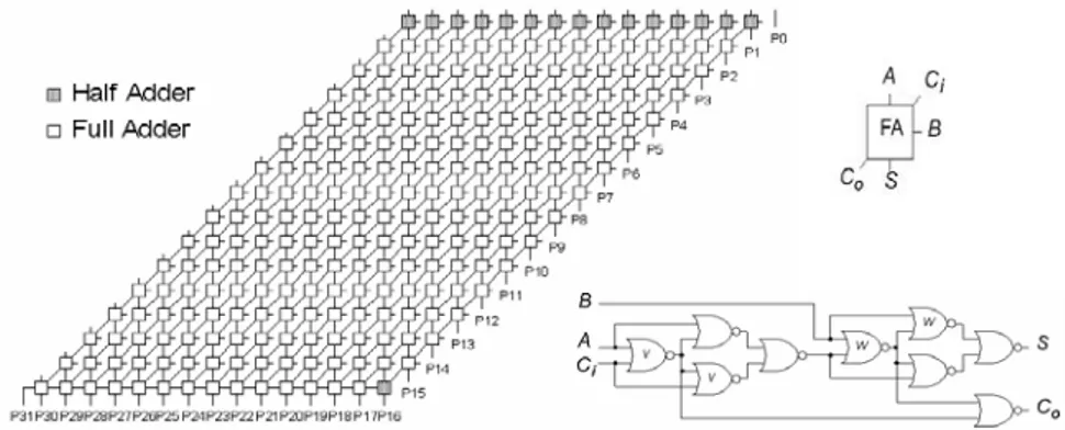
Here we explore various LP approaches to model-based diagnosis, and apply them to the c6288 digital circuit from the ISCAS’85 set of bench-marks4. C6288 (Fig. 1) is a 16-bit multiplier, which can be seen as a grid-like
pattern of 240 half and full adders, consisting of 2406 logical gates in all.
Figure 1. High-level Model of c6288 Multiplier Circuit and full adder module (images ob-tained from http://www.eecs.umich.edu/~jhayes/iscas/ ).
C6288 is of special interest in that it has traditionally proven difficult to diagnosis system. It is reported5 that several special-purpose diagnosers
could not reliably detect faults in this circuit. However, the best LP ap-proaches reliably detect all faults, and appear superior in the execution times. Moreover, LP approaches, when compared to the special-purpose ones, also have the advantage of requiring a very small amount of code – often less than a hundred lines.
In our experiments, we adopt the usual stuck-at fault model, where faulty circuit gates can be either stuck-at-0 or stuck-at-1, respectively outputting value 0 or 1 independently of the input. We first experimented with two na-ïve approaches that use a generation mechanism to identify possible sets of faults and then a test mechanism to test whether the faults are consistent with a given set of observations. We then experimented an approach that uses ta-bling to abduce faults consistent with observations. Here, for lack of space,
we only briefly mention them, though details can be found in a report6. We
then present an approach based on generating diagnoses as a stable model (SM) of a program, an approach that uses a novel mechanism of grounding the input to the SM generator via tabling. We next show how a deductive dependency-directed technique can be adapted to efficiently derive diagno-ses and be advantageously implemented in Prolog in a backtrack-free man-ner. Finally, we compare the performance of all techniques and analyse their strengths and weaknesses.
2. NAÏVE
APPROACHES
AND
TABLING
Perhaps the simplest, even naïve, method to test a circuit for a diagnosis is a simple generate-and-test method. Essentially, for each faulty gate that we intend to test, we simply replace its model by fixing its output to the ap-propriate faulty value which, in our running example is the negation of the correct value – generate phase. We then compare the output produced by the faulty model with the observed output. If they are the same, the (possible) fault is accepted, otherwise rejected – test phase. A slightly different method (that we call generate-and-check) consists in, rather than only comparing to the output vector in the end, to force the output vector in the test phase.
An alternative is a backtracking approach, making use of the in-built depth-first search strategy of Prolog engines. Instead of taking as input the faulty state of the gate, this approach simply models all the possible states of the gate, and returns either a list with the faulty state or an empty list.
The use of tabling is natural for handling the grid-like structure of c6288, which can require a huge amount of recomputation of circuit values, if a top-down approach (such as each of the two above) is used. In the tabling ap-proach, that we implemented in XSB7, we represent the faulty behaviour of a
gate as an assumption, and a diagnosis as a consistent set of assumptions.
3.
STABLE MODEL PROGRAMMING
A new, and growing in importance, LP paradigm is that of Stable Models (or Answer-set) Programming8,9. In it, solutions to a problem are represented
by the stable models10 of the corresponding program, rather than by answer substitutions of a single model of the program, as in traditional LP. In tradi-tional LP (as in the above) the diagnoses of a circuit are represented by terms, the clauses of the program being viewed as their recursive definition. In stable model (SM) programming, clauses are viewed as constraints on the diagnoses, each diagnosis being represented by a model of the program
de-fined in terms of those constraints. As claimed8, “stable model programming
is especially well suited for all problems where solutions are subsets of some universe, as each solution can be modelled by a different stable model”. This is definitely the case of circuit diagnosis, where solutions are subsets of abnormal gates, and so we have also used this new approach to solve the cir-cuit problem.
To represent our circuit diagnosis problem in SM programming, all we have to define is a suitable set of constraints over the predicates that define the circuit and the diagnoses. An important constraint in this domain is that each gate is either normal or abnormal, and cannot be both. This is easily coded by the following two rules:
abnormal(X) :- gate(X), not normal(X). normal(X) :- gate(X), not abnormal(X).
i.e. if X is a gate that is not normal then it must be abnormal, and vice-versa. Moreover, if some, e.g., AND-gate is normal, then its output value must be the conjunction of its inputs. If it is abnormal, its output is the negation of the conjunction. Rules imposing exactly this are:
val(out(and2,G), V):- normal(G), val(in(and2,G,1), I1), val(in(and2,G,2), I2), and(I1,I2,V). val(out(and2,G),V):- abnormal(G), val(in(and2,G,1), I1), val(in(and2,G,2), I2), nand(I1,I2,V).
It remains to be imposed that: a) no point can simultaneously have 2 dif-ferent values; b) all values of a given output vector are observed; and c) only single-faults occur:
inconsistent :- val(P,V1), val(P,V2), V1 \= V2.
explains :- val(out(and2,c545gat),V1), ..., val(out(nor2,c6288gat),V32). nonsingle :- abnormal(G1), abnormal(G2), G1 \= G2.
goal :- explains, not inconsistent, not nonsingle. :- not goal.
where each Vi in the explains/0 clause is replaced by the output value of the corresponding gate in a given output vector. This clearly resembles the for-mulation of an abduction problem: our goal is that all observed output values are explained, there are is inconsistency and no diagnoses with more than one abnormal gate. And we are only interested in SM’s in which our goal is satisfied (i.e. it is not false). The SM’s of this program, restricted to predicate abnormal/1, exactly correspond to the diagnosis of the circuit.
For computing the SM’s of the described program (i.e. the single-fault diagnoses of the circuit) we have used the smodels system11 version 2.26 for
Windows. For dealing with the grounding of the program, required by smod-els, and for pre-processing away the function symbols out/2 and in/3 used in the representation of the circuit, we have developed an XSB-Prolog pro-gram. Although this is all that is required of the XSB-Prolog for this circuit
diagnosis problem, the program does more. The additional functionality of the mentioned XSB-Prolog program might be crucial for other diagnosis problems and, in general, for other problems that can be coded as abduction.
Our XSB-Prolog program starts by running the query goal in a program with the representation of the problem having the above clause for goal/0, without the last clause (:- not goal), and where all predicates are tabled. In this
execution, all calls that depend on loops over negation are suspended. Note that, in the above representation, the only loop over negation is the one be-tween predicates abnormal/1 and normal/1. After the execution, the tables of the various predicates contain the so-called residual program11, which has,
for each predicate, the (non-failing) rules used during execution, simplified by removing all body literals proven true (and not suspended). It is well known11 that the SM’s of the residual program are the same as those of the
part of the original program relevant to the query. Moreover, if all the calls during the execution are ground (which is the case for our representation) the residual program is also ground. Thus, this residual program, after some simple pre-processing that eliminates the function symbols out/2 and in/3, is what is passed to smodels for computing the diagnoses. This method is now easy to implement, due to the recent XAsp package of XSB 2.6, which al-ready provides special predicates for this purpose and linking to smodels. Its main advantage over a direct usage of smodels is that only the part of the program relevant to the query has to be considered when computing the SM’s. Besides gains in efficiency, this is also important for general abduc-tion problems: in this way, the obtained abductive soluabduc-tions come only in terms of abducibles relevant to the query (i.e. only relevant abductive solu-tions are computed).
4. DEPENDENCY-DIRECTED DIAGNOSIS
As an alternative to model the circuit diagnosis problem, we represent digital signals with sets and Booleans. A deductive dependency-directed technique13,14 is used to simulate the circuit behaving normally, as well as to deduce the behaviour of all faulty circuits. This technique has been used by the Electronic CAD community for fault simulation, but in this section we show how to apply it to our diagnosis problem.
Since the faulty behaviour of a circuit can be explained by several sets of faults, we represent a signal not only by its normal value but also by the set of diagnoses it depends on. More specifically, a signal is denoted by a pair L-N, where N is a Boolean value (representing the Boolean value of the cir-cuit when there are no faults) and L is a set of diagnoses, that might change the signal into the opposite value. For instance, for single faults,
X={g/0,i/1}-0 means that signal X normally is X={g/0,i/1}-0 but if gate g is stuck-at-X={g/0,i/1}-0, or gate i is stuck-at-1, then its actual value is 1. ∅-N represents a signal with constant value N, independently of any fault. For generality, we need to explicitly represent the fault modes in the set of faults. In the following we assume that any gate in a circuit may be faulty.
A gate g, that can either be normal, stuck-at-0 or stuck-at-1, may be mod-elled by means of a normal gate to which a special buffer, an S-buffer, is at-tached to the output. As such, all gates are considered normal, and only S-buffers can be faulty. The modelling of S-S-buffers is as in Table 1:
Table 1. S-buffer logic table
In ∅-0 ∅-1 Li-0 Li-1
Out {g/1}-0 {g/0}-1 {g/1} ∪ Li - 0 {g/0} ∪ Li - 1
When the input is 0 and independent of any fault, the S-buffer output would normally be also 0, but if it is stuck-at-1 then it becomes 1. More gen-erally, if the normal input is 0 but dependent on Li, the output depends not
only on g/1 but also on input dependencies Li. The same reasoning can be
applied to the case where the normal input signal is 1, and the output of an S-buffer g with input Li-N can be generalised to {g/N}∪Li-N, where N stands
for the complement of Boolean value N.
Normal gates fully respect the Boolean operation they represent. We dis-cuss the behaviour of NOT and AND-gates as illustrative of these gates. All other gates can be modelled as combinations of these. Given the above ex-planation of the encoding of digital signals, for a normal NOT-gate whose input is signal L-N, the output is simply L-N, since the set of faults on which it depends is the same as the input signal.
For an AND-gate, in the absence of faults, the output is the conjunction of the normal inputs. The set of faults that may change the output signal into the opposite of the normal value is less straightforward to determine. When both normal inputs are 1 (1st case of the table below), a fault in set L1 or set
L2 justifies a change in the output. In the second case (two 0s), to invert the
output signal, a fault in both L1 and L2 must exist. So, the set of faults that
justify a change in the gate's output is the intersection of the input sets. In the last two cases, to obtain an output different from the normal 0 value, it is necessary to invert the normal 0 input, and not to invert the normal 1 input (justifying the set difference in the output), as in Table 2:
Table 2. AND-gate logic table
In1 L1-1 L1-0 L1-0 L1-1
In2 L2-1 L2-0 L2-1 L2-0
To model the diagnosis problem and find the possible single faults that explain the faulty output vector F, a bit-wise comparison between F and the deduced simulated logic output must be performed. Let ro and so denote,
re-spectively, the real and simulated value of output bit o, where ro is a Boolean
value Bo and so is a set-Boolean pair Lo-No. When Bo≠ No, the only possible
single faults are in Lo and any such fault explains Bo. When Bo = No, none of
the faults in Lo occur. Hence, the set of faults that justify the full incorrect
output vector F is given by {f: ∀o ((Bo≠ No⇒ f ∈ Lo) ∧ (Bo = No⇒ f ∉ Lo))}
where o ranges over all the output bits. The diagnostic solution is then given by intersecting all the dependency sets Lo where ro is incorrect and removing
the union of Lo where ro is as expected.
The LP implementation of the dependency-directed fault diagnosis is immediate: we simply propagate bottom-up the signals over the circuit (as in the generate-and-test, and backtracking approaches), making use of logical variables and unification. In contrast with the generate-and-test implementa-tion, Boolean values representing 0/1 circuit values are now substituted by a term Value-ListOfGates, and the gates' behaviours are as described above. To implement the set operations, we resorted to the ordsets library for opera-tions over sorted lists of SICStus Prolog15. Of all the approaches in this
pa-per, it turns out that this is the most efficient one. This is as expected, since with this approach only one pass in the circuit is needed to extract the infor-mation needed to compute all the faults for all the output vectors.
This method can be extended to handle multiple fault diagnoses. The ma-jor problem is the representation of all the possible diagnoses. In the single fault case, our sets may have at most 2*G gates, where G is the number of gates in the circuit (2406 for c6288). However, for double faults the lists may expand to 4*G2 (around 23 million elements for c6288!). A better
rep-resentation is needed in order to avoid this explosion. We tried to encode sets of double faults by sets of pairs of the form (f,ListOfFaults) or (f,-ListOfFaults). For instance, the pair (10/1,[20/0,40/1,50/1]) represents the set of faults {(10/1,20/0), (10/1,40/1), (10/1,50/1)}, while (10/1,-[20/0,40/1,50/1]) stands for the set of all double faults, containing 10/1, mi-nus the above ones. We have extended the ordinary set operations to pairs of this form and tested it with c6288. All double faults for c6288 could be de-termined in a reasonable amount of time (see the conclusions section).
5. RESULTS
AND
CONCLUSIONS
In this paper we addressed several approaches to the circuit diagnosis problem. The implementations were tested using the same input vector, 01001000000100010001000110100000, corresponding to the multiplication
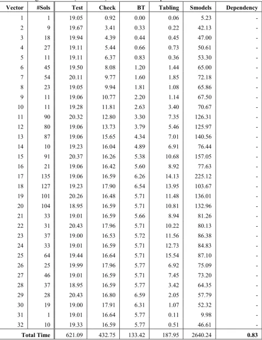
of 34834 by 1416, returning 49324944, represented in binary by (least sig-nificant bit first) 00001001110001010000111101000000. From this correct output we flipped a bit at a time, obtaining 32 incorrect output vectors. The results for the various approaches were as shown in Table 3 (all tests run on a Pentium III 733 MHz; for Test, Check, BT and Dependency, SICStus 3.8.5 was used; for Tabling, XSB-Prolog 2.2; for Smodels, SModels 2.26):
Table 3. Diagnosis results (in seconds) for 32 incorrect ouput vectors of c6288.
Vector #Sols Test Check BT Tabling Smodels Dependency
1 1 19.05 0.92 0.00 0.06 5.23 - 2 9 19.67 3.41 0.33 0.22 42.13 - 3 18 19.94 4.39 0.44 0.45 47.00 - 4 27 19.11 5.44 0.66 0.73 50.61 - 5 11 19.11 6.37 0.83 0.36 53.30 - 6 45 19.50 8.08 1.20 1.44 65.00 - 7 54 20.11 9.77 1.60 1.85 72.18 - 8 23 19.05 9.94 1.81 1.08 65.86 - 9 11 19.06 10.77 2.20 1.14 67.50 - 10 11 19.28 11.81 2.63 3.40 70.67 - 11 90 20.32 12.80 3.30 7.35 126.31 - 12 80 19.06 13.73 3.79 5.46 125.97 - 13 87 19.06 15.65 4.34 7.01 140.56 - 14 10 19.23 16.04 4.89 6.91 76.44 - 15 91 20.37 16.26 5.38 10.68 157.05 - 16 21 19.06 16.42 5.60 8.92 77.63 - 17 135 19.06 16.59 6.26 14.13 225.12 - 18 127 19.23 17.90 6.54 13.95 103.67 - 19 101 20.26 16.48 5.71 11.48 136.01 - 20 104 18.95 16.59 5.71 10.81 132.96 - 21 33 19.01 16.59 5.66 8.94 81.26 - 22 31 20.43 17.96 5.71 10.22 80.13 - 23 37 19.00 16.53 5.72 11.56 86.38 - 24 33 19.01 16.59 5.71 12.73 84.83 - 25 64 19.44 16.64 5.71 15.54 87.10 - 26 25 19.99 17.96 5.77 6.92 75.09 - 27 46 19.01 16.59 5.71 7.45 73.20 - 28 37 18.95 16.59 5.77 3.42 64.35 - 29 28 20.43 16.80 6.59 2.05 57.79 - 30 19 19.00 17.91 6.31 1.07 52.32 - 31 1 19.01 16.64 5.77 0.11 9.98 - 32 10 19.33 16.59 5.77 0.51 46.61 - Total Time 621.09 432.75 133.42 187.95 2640.24 0.83
Timings should be looked with some care. Note that we are using differ-ent Prolog systems, with possible impact on the performance. In the last col-umn of the table, only the total time appears since, for the dependency-directed approach, the information needed to obtain the diagnoses is com-puted in a single propagation over the circuit (this phase takes 220ms). The diagnoses for each test are then obtained by set operations on the results, this phase taking a total of 610ms. On average, for a single test vector, diagnoses can be found in around 20ms, after propagation. Thus, total execution time reduces to 240ms. This is by far the best method presented here. The main reason is that, contrary to previous methods, this one is backtrack-free. The method can also be generalized to multiple faults. When computing all dou-ble faults, the propagation phase took approximately 780 seconds. Note that the operations on sets of faults are now more complex and therefore we have a 3500-fold slowdown. An implementation for larger cardinality of faults is an open research problem. Notice that a similar technique can be used in Abductive LP, widening the applications of the method.
As expected, generate-and-test takes constant time. Generate-and-check is a little better, but its performance degrades as the wrong bit becomes more and more significant, since incorrect assumptions fail later. The backtracking version performs quite well, but shows the same problem of generate-and-check, for the same reasons.
The tabling approach is very good at solving problems with a small num-ber of faults, the running times being almost independent of the wrong bit. The justification is a dynamic ordering of inputs and dependencies checking used to direct the search. It gets worse for greater number of faults since more memory is required to store the tabled predicates. Also notice that XSB Prolog is much slower than SICStus.
The SM programming approach is, among those presented, the least effi-cient. However, this approach has been specially tailored for solving NP-complete problems, which is not the case for our single-fault circuit diagno-sis. Nevertheless, we were impressed with the robustness of the smodels sys-tem, which was capable of handling the very large files resulting from the residual program for each test in this circuit. In fact, for each output vector, the (ground) logic program, generated by the XSB-Prolog program, that served as input to smodels has, on average, 31036 clauses and around 2.4 MB of memory. On the other hand, the representation of the circuit and of the problem is (arguably) the most declarative and easier one.
We have also tried to implement a solution resorting to SICStus library of constraints over Booleans. Our efforts proven useless, since SICStus was unable to handle the constraints we generated (usually, ran out of memory).
Although we did not run specialized diagnosis systems in the same plat-form, we can compare our times with the ones presented by those systems
some years ago, and take into account the hardware evolution. The results of the shown LP approaches are then quite encouraging. For example, the re-sults of the DRUM-II specialized system16 seem worse than ours: it can take
160 seconds to diagnose all single faults in c6288 for a specific output vec-tor. We dare to say that this system, even if ported to an up-to-date platform, would still be less efficient than our dependency-directed approach (which takes 0.83s to produce the diagnoses for the 32 output vectors), and would possibly be comparable to our general approaches of backtracking and tabu-lation (which, for the worst case take, respectively, 6.59 and 15.54 seconds).
REFERENCES
1. P. Lucas, Symbolic Diagnosis and its Formalisation, The Knowledge Engineering Review 12(2), (1997), pp. 109−146.
2. J. Doyle, A Truth Maintenance System, Artificial Intelligence 12(3), (1979), pp. 231-272. 3. J. de Kleer and B. C. Williams, Diagnosing Multiple Faults, Artificial Intelligence 32(1),
(April 1987), pp. 97-130.
4. ISCAS. Special Session on ATPG, Proceedings of the IEEE Symposium on Circuits and
Systems, Kyoto, Japan, (July 1985), pp. 663−698.
5. P. Fröhlich, DRUM-II Efficient Model-based Diagnosis of Technical Systems, PhD thesis, University of Hannover, (1998).
6. J. J. Alferes, F. Azevedo, P. Barahona, C. V. Damásio and T. Swift, Logic Programming Techniques for Solving Circuit Diagnosis; ssdi.di.fct.unl.pt/~fa/papers/diagnosis_ps.zip. 7. The XSB Programmer's Manual: version 2.1, Vols. 1-2 (2000); http://xsb.sourceforge.net 8. M. Marek and M. Truszczyński, Stable models and an alternative logic programming
paradigm, The Logic Programming Paradigm: a 25-Year Perspective, (Springer, 1999), pp. 375−398.
9. I. Niemelä, Logic programs with stable model semantics as a constraint programming paradigm, edited by I. Niemelä and T. Schaub, Computational Aspects of Nonmonotonic
Reasoning, (1998), pp. 72−79.
10. M. Gelfond and V. Lifshitz, The stable model semantics for logic programming, in:
ICLP'88, edited by R. Kowalski and K. Bowen (MIT Press, 1988), pp. 1070−1080. 11. I. Niemelä and P. Simons, Smodels - an implementation of the stable model and
well-founded semantics for normal logic programs, in: 4th LPNMR, (Springer, 1997).
12. W. Chen and D. S. Warren, Computation of stable models and its integration with logical query evaluation, IEEE Trans. on Knowledge and Data Engineering (1995).
13. D. B. Armstrong, A Deductive Method of Simulating Faults in Logic Circuits, IEEE
Trans. on Computers C-21(5), 464−471 (May 1972).
14. H. C. Godoy and R. E. Vogelsberg, Single Pass Error Effect Determination (SPEED),
IBM Technical Disclosure Bulletin 13, 3443−3344 (April 1971).
15. Programming Systems Group of the Swedish Institute of Computer Science. SICStus
Prolog User’s Manual, (1995).
16. Peter Fröhlich and Wolfgang Nejdl, A static model-based engine for model-based reason-ing, in: Proceedings of IJCAI97 (1997), pp. 466−473.