A Work Project presented as part of the requirements for the Award of a Master’s Degree in Finance from the NOVA - School of Business and Economics
Dissecting the Determinants of Inflation in the US
Ricardo Henrique Lopes Correia, 29739
A project carried out in the Master’s in Finance Program, under the supervision of:
Professor Martijn Boons
2
Abstract
This paper studies the determinants of inflation in the US under a VAR modeling approach,
using Granger causality tests and out-of-sample performance comparisons, to provide a deeper
analysis for asset management. It is demonstrated that after correcting for structural changes,
both money supply and real activity measures have merit in determining inflation. More
importantly, the paper shows how decisive it is for asset managers to understand the ways
structural changes affect these traditional transmission mechanisms and how to take them into
account in order to be able to timely assess inflation trends.
3
Introduction
Inflation is a phenomenon of great importance to all economic agents, as a general price
increase, or decrease, has repercussions on several dimensions, from consumer purchasing
power and savings to debt burdens and competitiveness of domestic products. Moreover, the
lack of price stability distorts its function of conveying supply and demand information, thus
perturbing economic decisions. Therefore, it is a crucial factor for asset managers, in particular
those managing longer term macro strategies. It is in such context that this paper, developed as
part of a Directed Research Internship with Banco de Investimento Global (BiG), aims to
provide a detailed analysis over several economic variables and relationships commonly used
to forecast inflation, in order to understand what truly drives inflation across macroeconomic
contexts. This necessity arises from the fact that different methods of forecasting, grounded on
various theoretical or empirical backgrounds, have performed differently through time,
signaling the importance of assessing how structural changes influence the inflationary process.
Such is accomplished by breaking down the transmission mechanisms of these relationships to
verify its theoretical validity in practice through an econometric analysis of causality, followed
by forecasting performance comparisons between a commonly used benchmark and the models
proposed in this paper, as additional confirmation. Ultimately, the intent is to provide insight
on the inflation drivers in the US to contribute to an informed and profitable asset allocation by
asset managers. In particular, it is an especially relevant topic at a time when inflation has been
interestingly low and stable in the last decade – despite several indicators pointing otherwise –
and at a time of highly sensitive monetary policy shifts.
The paper is structured as follows: a literature review covering the timeline of forecasting
methods that sets up consequent hypotheses (pp. 4-7); a specific focus on the relationship
4 7-12); an empirical analysis of relevant relationships (pp. 13-20); and finally a discussion and
closing remarks (pp. 20-22).
Literature review
The literature on this topic is vast, covering different forecasting approaches that stem from a
disagreement on what truly causes inflation. Various schools of thought have formulated
theories of inflation, with the main strands being either Keynesian or Monetarist inspired.
Keynesian schools posit that inflation can result from excessive aggregate demand growth
relative to aggregate supply growth – demand-pull inflation –, from a supply shock due to
higher costs of production – cost-push inflation –, and from expectations that past inflation will
persist coupled with the price/wage spiral – built-in inflation (Gordon, 1988). Monetarist
schools, on the other hand, describe inflation as an event originating from greater money supply
growth relative to output growth, and thus, as an exclusively monetary phenomenon (Friedman,
1963). Because of this, several model specifications have been proposed to forecast inflation,
most of which showing inconsistent performance across sample periods and inflation measures.
Papers such as Stock and Watson (1999) demonstrate the predictive reliability of Phillips curve
specifications, an approach based on empirical observation by Phillips (1958) that uses real
activity measures to forecast inflation, for one-year-ahead forecasts compared to a simple
univariate benchmark. Notably, the authors demonstrate the superior performance of using a
Phillips curve model based on a composite activity index, as well as no advantage from
including money supply measures. Several critics to Phillips curve predictive capabilities have
been documented in the literature, a peremptory example of such being Atkeson and Ohanian
(2001), which compares textbook NAIRU and Stock and Watson (1999) specifications with a
random walk model on 12-month inflation and finds superior performance of the naïve
5 finds that this relationship has changed over time with correlations peaking during recessions
and shocks to inflation being rather persistent, especially since the 1990s, when Phillips curve
specifications started to lose their predictive power. Furthermore, it finds that the sharper the
shock to inflation, the longer its effects will influence price levels – such was the case for the
last financial crisis. The breakdown of this correlation, on the other hand, appears mostly during
recoveries, when both high unemployment and high productivity and prices coexist (Quévat
and Vignolles, 2018). Smets and Wouters (2007) argue that such behavior is likely due to lower
volatility of shocks themselves, rather than due to fundamental changes, which indicates a need
to observe stronger real activity oscillations before it is possible to verify its repercussions on
price level. It has been, in fact, extensively noted in the literature that conventional Phillips
curve relationships have weakened since the 1990s. Some papers have verified this widespread
idea that the Phillips curve has flattened between the 1970s and 1990s, and remained stable
since then (Blanchard, Cerutti and Summers, 2015). Importantly, Stock and Watson (2008)
recognize the univariate model superiority in forecasting but show evidence of the relevance of
equating real activity measures to inflation at turning points – at which we are presently. This
point highlights the crucial need to understand what fundamentally drives inflation across
structural shifts and that univariate outperformance is likely to be circumstantial rather than
ultimately superior. For instance, some of the opposition to Phillips curve models is based on
an apparent decoupling of productivity and wage growth since the 1990s. Schwellnus, Kappeler
and Pionnier (2017) argue that when correcting for greater wage inequality and decreasing labor
share, this decoupling is no longer present. Moreover, Anderson (2007) substitutes the
commonly used average hourly earnings measure by total compensation, to reflect increased
relevance of variable pay relative to base salary in recent history, and finds a closer proximity
between both variables. Quévat and Vignolles (2018) further include productivity to enrich
6 The role of money in forecasting, in turn, is still upheld by a solid body of literature. In
particular, authors argue for not only high correlation at low frequencies, but also leading
properties of money over inflation in low frequency data for longer-term forecasts, defending
its predictive value (Assenmacher-Wesche and Gerlach, 2008a, 2008b; Azevedo and Pereira
2010; Lanne, Luoto and Nyberg, 2014). The long run predictive power of money measures is
widely accepted, but its usefulness in short run forecasting is a subject of debate. Papers such
as Woodford (2007a) and Binner et al. (2009), argue that monetary aggregates either have no
predictive power or improvements based on them are only marginal compared to simple random
walk models. The latter refers to Atkeson and Ohanian (2001) in search for an explanation for
this pattern, citing the difficulty of forecasting not only inflation, but also various other
economic variables since the 1980s, proposing also an alternative reasoning – that monetary
aggregates may be less informative when inflation is low and stable.
Despite the above mentioned findings, Ang, Bekaert and Wei (2007) conducted a large
comparative analysis of forecasting models, from simple random-walk models to Phillips curve
specifications and combined forecasts, and found that survey data outperforms all other
specifications for CPI measures, whereas PCE measures were shown to follow simple
random-walk specifications, and in both cases, Phillips curve models were outperformed. This study
was mostly done through simple linear regression analysis using OLS and for one-year ahead
forecasts. In order to mitigate the apparent inconsistency, combined forecasts and alternative
methods have also been tested, from simple means to time-varying parameters and Bayesian
dynamic model averaging (Koop and Korobilis, 2009), as well as bagging methods (Inoue and
Kilian, 2007).
Overall, all methods appear to be very unreliable for definitive usage, indicating that the
7 because of this uncertainty in modeling inflation that this paper attempts to provide a robust
fundamental analysis of the main inflation drivers to reinforce econometric forecasts.
Determinants of Inflation
On Money Supply
The emphasis on monetary aggregates started to give way to other methods of inflation
forecasting in the late 1980s, where a disconnection between money supply growth and inflation
first became apparent. Up until then, excess money growth was highly correlated and exhibited
a leading relationship with inflation over longer horizons, a relationship that since then has
broken down. This can be broadly demonstrated by plotting 10-year moving averages of both
variables, with 1990 as the turning point (Chart 1). Specifically, correlations between long
averages of excess money growth and inflation measures up to the 1990s were as high as 91%,
before heavily inverting since then – although for the whole sample correlations are still
relevant, standing around 60%. Velocity of money, which had been fairly stable until then, also
started exhibiting a much more unpredictable behavior precisely when the connection appears
to have diverted – an argument used by opponents of traditional Monetarism, as stable velocity
is one of its assumptions – which can also be seen in Chart 1.
Testing these relationships with different money definitions – such as MZM – leads to similar
conclusions, as the bulk of these aggregates are measures shared by all of them. However, it
can be argued that money has become increasingly hard to define as innovations in the financial
markets have made it difficult to distinguish what truly is money used in real economy
transactions. Said phenomenon may be attributed in part to an increasing relevance of the
financial sector and, recently, to the subdued effect of the Fed’s extra liquidity on prices. With
increased financial sector preponderance, there is a larger money leakage to the financial system
8 pattern: the financial sector has since the 1980s surged in percentage of total GDP, as financial
innovations attracted more and more capital, incentivized leveraging and contributed to asset
price surges that are not captured by standard inflation measures, based on goods and services.
In itself, this pattern should not translate into a real economy deceleration, on the contrary, it
should contribute to faster and broader investment throughout non-financial sectors. However,
data shows a growing gap of financial to real assets (Chart 2, as a ratio of financial to total
assets), a factor that is coupled with higher industry concentration and market power that leads
to higher profit margins without increasing productivity – aspects that will be covered in the
next section.
It is possible to visualize this phenomenon by looking at measures such as velocity of money
or money multipliers. Assumed to be stable in the equation of exchange1, velocity of money is
a good indicator of imbalances in the transmission mechanism from money supply to prices. In
fact, and giving special attention to the unprecedented increase in money supply since the great
financial crisis, a large part of the extra liquidity from quantitative easing has remained within
the money market. Theory would indicate that increasing money supply should increase banks’
reserves, which in turn reduces the federal funds rate since demand for money is lower and
supply is larger. With lower costs of capital, banks should be extending more credit,
contributing to more spending and investment, and consequently, inflation. On the contrary,
banks have retained much of this extra liquidity as excess reserves – to levels without historical
precedent that have remained high since the beginning of quantitative easing, in large due to
interest payments by the Fed on these reserves –, and have been notably more conservative in
extending credit – delinquency rates on credit card loans, for instance, dropped to historical
lows –, thus having a minimal effect on inflation. The diminished effect could also come from
a higher personal saving rate – or money hoarding –, however, data shows the personal saving
9 rate at relatively low levels. Velocity of money therefore reflects this, continuing the steady
decline since the 1990s, with a large drop during the last crisis, as well as the various money
multipliers – money stock measures such as M2 divided by the Monetary Base – which have
similarly reached all-time lows.
In conclusion, it is hypothesized that it is not that money has no longer a tight connection with
inflation, but rather that it is harder to measure effective money supply today than back in the
height of Monetarism, and that recent increases in the monetary base have not translated into
more available money for the real economy. For modeling purposes, the hypothesis is that we
can use the velocity of money as a proxy of the imbalances in the theoretical money supply
relationship with inflation, attaining stronger causality than with excess money growth as a sole
predictor – as demonstrated in the Empirical Analysis section.
Chart 1 – 10Y Moving Avg. of Excess M2 Growth and CPI inflation rate (Velocity on secondary axis)
Source: Author’s calculations using FRED data
0.0 0.5 1.0 1.5 2.0 2.5 0% 1% 2% 3% 4% 5% 6% 7% 8% 9% 10% 1 9 6 9 -1 0 1 9 7 1 -0 7 1 9 7 3 -0 4 1 9 7 5 -0 1 1 9 7 6 -1 0 1 9 7 8 -0 7 1 9 8 0 -0 4 1 9 8 2 -0 1 1 9 8 3 -1 0 1 9 8 5 -0 7 1 9 8 7 -0 4 1 9 8 9 -0 1 1 9 9 0 -1 0 1 9 9 2 -0 7 1 9 9 4 -0 4 1 9 9 6 -0 1 1 9 9 7 -1 0 1 9 9 9 -0 7 2 0 0 1 -0 4 2 0 0 3 -0 1 2 0 0 4 -1 0 2 0 0 6 -0 7 2 0 0 8 -0 4 2 0 1 0 -0 1 2 0 1 1 -1 0 2 0 1 3 -0 7 2 0 1 5 -0 4 2 0 1 7 -0 1
10
Chart 2 – Financial Assets to Total Assets of Nonfinancial Business, Households and Nonprofits
Source: Author’s calculations using FRED data
On Real Activity
Traditional Phillips curve specifications establish a relationship between inflation, past
inflation, unemployment gap and variables to control for supply shocks. However, in a broader
sense, it is any relationship between real aggregate activity and inflation (Stock and Watson,
1999). As discussed in the literature review above, many Phillips curve specifications have been
supported and refuted, and as such, in this paper an attempt is made to deconstruct the most
commonly tested relationships to determine whether they are ultimately useless or if they have
simply suffered structural changes that need to be accounted for.
Starting with the most well-known relationship, this paper studies unemployment and inflation.
The way this relationship takes place relates to wage growth, capacity utilization and
productivity. In theory, when the economy is highly productive, operating near maximum
capacity and unemployment reaches significantly low levels – below the NAIRU – there is an
upward pressure on wages, which then translates into an upward pressure on inflation through
50% 52% 54% 56% 58% 60% 62% 64% 66% 1 9 5 1 -1 0 1 9 5 4 -0 2 1 9 5 6 -0 6 1 9 5 8 -1 0 1 9 6 1 -0 2 1 9 6 3 -0 6 1 9 6 5 -1 0 1 9 6 8 -0 2 1 9 7 0 -0 6 1 9 7 2 -1 0 1 9 7 5 -0 2 1 9 7 7 -0 6 1 9 7 9 -1 0 1 9 8 2 -0 2 1 9 8 4 -0 6 1 9 8 6 -1 0 1 9 8 9 -0 2 1 9 9 1 -0 6 1 9 9 3 -1 0 1 9 9 6 -0 2 1 9 9 8 -0 6 2 0 0 0 -1 0 2 0 0 3 -0 2 2 0 0 5 -0 6 2 0 0 7 -1 0 2 0 1 0 -0 2 2 0 1 2 -0 6 2 0 1 4 -1 0 2 0 1 7 -0 2
11 demand-pull. In the literature review above, various authors were mentioned with respect to
modifications in this simple relationship in order to account for structural changes over time.
These are taken into consideration in order to improve the analysis. In a similar way to what
was done for money supply measures, some hypothesis related to real activity specifications
are stipulated beforehand, that are then tested in the Empirical Analysis section, combining all
of these insights from the literature.
The markedly reduced impact of real activity on price levels is hypothesized in this study to be
related to low productivity growth levels and consequently modest wage growth, as well as to
labor market trends with respect to worker distribution per sector. Low productivity growth
levels in the US have been a trend in recent years that can be attributed to a decrease in corporate
investment in tangible and knowledge-based capital, which in turn is likely to derive from an
uncertain policy environment and constraints on the housing and credit markets. Corporate
investment has dropped all across developed countries and has showed a very modest recovery,
with much of the US business community focusing on less asset-heavy sectors – a fact that,
while partly due to technology sector growth, can be attributed to less confidence in the business
environment. Furthermore, industry concentration has been growing since the 1990s, with
lower competition between firms and larger chunks of market share flowing to fewer groups.
This consolidation, in turn, leads to the high profit margins that have been recorded recently,
but which do not derive from increased productivity (Chart 3). Adding to this scenario is the
labor force trend, which shows a decrease in labor force participation due to ageing population,
and a shift of added jobs towards low productivity sectors such as Healthcare and Social
Assistance. The recent low productivity scenario may also be connected with the money market.
With more conservative credit policies and greater emphasis on the short term by corporations,
12 financial crisis is only slowly corrected and companies invest less in riskier, more disruptive
projects.
Other factors that signal overheating in an economy are capacity utilization and the
unemployment gap. In the US, capacity utilization has been peaking at consistently lower levels
since the 1970s and the unemployment rate is just now dropping below the consensual long run
sustainable level. When these variables stay off their overheating levels, real activity does not
impact inflation as much, given the incentive to continue hiring before there is an upward
pressure on wages.
In the section below, an econometric analysis is developed on the hypothesis presented above
using insights from the literature review.
Chart 3 – Smoothed Annual Labor Productivity Growth (5Y Moving Avg.)
Source: Author’s calculations using FRED data
0.0% 0.5% 1.0% 1.5% 2.0% 2.5% 3.0% 3.5% 4.0% 4.5% 1 9 5 2 -1 0 1 9 5 5 -0 2 1 9 5 7 -0 6 1 9 5 9 -1 0 1 9 6 2 -0 2 1 9 6 4 -0 6 1 9 6 6 -1 0 1 9 6 9 -0 2 1 9 7 1 -0 6 1 9 7 3 -1 0 1 9 7 6 -0 2 1 9 7 8 -0 6 1 9 8 0 -1 0 1 9 8 3 -0 2 1 9 8 5 -0 6 1 9 8 7 -1 0 1 9 9 0 -0 2 1 9 9 2 -0 6 1 9 9 4 -1 0 1 9 9 7 -0 2 1 9 9 9 -0 6 2 0 0 1 -1 0 2 0 0 4 -0 2 2 0 0 6 -0 6 2 0 0 8 -1 0 2 0 1 1 -0 2 2 0 1 3 -0 6 2 0 1 5 -1 0 2 0 1 8 -0 2
13
Empirical Analysis
In this section, data description, summary statistics and stationarity tests are presented for all
variables used in econometric analysis, then separate causality tests are conducted regarding
money supply measures and real activity measures, leading to the specification of a few models
based on the conclusions drawn beforehand, and finally to an out-of-sample performance
comparison between the proposed models and a common benchmark.
Data and Summary Statistics
All data series used directly or posteriorly manipulated by the author are collected from the
Federal Reserve Economic Data (FRED) website. The data has quarterly frequency and a
maximum sample size of 282 observations, corresponding to 1948Q1:2018Q2. As a measure
of the relevant variable – inflation rate – the Consumer Price Index (CPI) is preferably used, as
there is a wider range of comparable forecasting methods based on it. The chosen measure of
money definition is the M2 monetary aggregate for similar reasons – widespread usage by
practitioners and the Fed. Two measures of wage growth are studied in order to assess
differences in base wage growth versus total compensation growth. All variables that constitute
percent changes are presented on a year-on-year basis – inflation, average hourly earnings and
total compensation growth, and excess M2 growth –, the remaining percent unit variables are
level – unemployment rate, capacity utilization and yield curve spread. Detailed information on
all variables can be found in Table 1.
Methodology
In this paper, the chosen method for modeling inflation is the Vector Autoregressive (VAR)
model, in which variables are arranged in a set of linear dynamic equations whose number is
the same as the number of variables, meaning each variable at a time is modeled as dependent – on an equal number of its own lags and lags of other variables. This method is useful to model
14 economic data in the sense that it captures intertemporal dependencies between variables,
allowing us to assess causality through structural changes. As a requirement to implement this
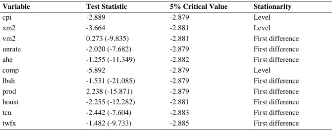
approach, it is necessary to ensure that variables enter the model in a stationary form, either
level or after differencing. To do so, the Augmented Dickey-Fuller Test (ADF) is run on each
variable, whose results can be found in Table 2. (Note that differenced variables will be prefixed
by a “d” from this point on.) As a base criteria for null hypothesis rejection, the 5% significance
level is used throughout the paper. Every test and modeling procedure presented along this
section is performed in STATA.
Table 1 – Data description and summary statistics
Variable Name Unit Obs Mean Std Dev Min Max
CPI Inflation Rate cpi % 282 3.51% 2.92% -2.79% 14.43%
Excess M2 Growth xm2 % 234 3.60% 3.15% -3.47% 12.75%
Velocity of M2 vm2 ratio 238 1.81 0.18 1.43 2.20
Unemployment Rate unrate % 282 5.78% 1.63% 2.57% 10.67%
Average Hourly Earnings ahe % 214 4.17% 1.97% 1.42% 9.10%
Total Compensation comp % 282 1.54% 1.67% -2.75% 5.35%
Labor Share lbsh index* 282 109.52 4.47 98.15 117.51
Labor Productivity Index prod index* 282 59.16 24.13 24.09 105.10 Housing Starts houst thousands 237 1432.70 391.08 525.67 2424.00 Total Capacity Utilization tcu % 206 80.27% 4.19% 67.12% 88.51% Trade-Weighted Exchange
Rate USD-Major
twfx index* 182 129.17 19.34 95.36 194.79
10Y-2Y Yield Spread spd % 168 0.96% 0.91% -1.28% 2.80%
*: 2012 as base year
Notes: Variables presented before modifications to enter econometric models. Source: Author.
Table 2 – Augmented Dickey-Fuller Tests
Variable Test Statistic 5% Critical Value Stationarity
cpi -2.889 -2.879 Level
xm2 -3.664 -2.881 Level
vm2 0.273 (-9.835) -2.881 First difference
unrate -2.020 (-7.682) -2.879 First difference
ahe -1.255 (-11.349) -2.882 First difference
comp -5.892 -2.879 Level
lbsh -1.531 (-21.085) -2.879 First difference
prod 2.238 (-15.871) -2.879 First difference
houst -2.255 (-12.282) -2.881 First difference
tcu -2.442 (-7.604) -2.883 First difference
15
spd -2.327 (-10.719) -2.886 First difference
Notes: A test statistic lower than the critical value means the null hypothesis of no stationarity is rejected. Test statistics between parentheses refer to test results after differencing.
Source: Author.
After ensuring stationarity, Granger causality tests are run on common model specifications
and on modified specifications that result from the hypotheses formulated above and from test
results, for the whole sample. In this phase, the analysis is once again segmented in money
supply measures and real activity measures. All tested models follow this generalized
specification for a multivariate VAR with 𝑝 lags:
𝑦𝑡 = 𝑐 + 𝐴1𝑦𝑡−1+ 𝐴2𝑦𝑡−2+ ⋯ + 𝐴𝑝𝑦𝑡−𝑝 + 𝑢𝑡 (1)
where each 𝑦𝑖, 𝑐 and 𝑢𝑡 are vectors of length equal to 𝑚 variables and 𝐴1, … , 𝐴𝑝 are 𝑚𝑥𝑚
matrices of coefficients for each lag 1, … , 𝑝.
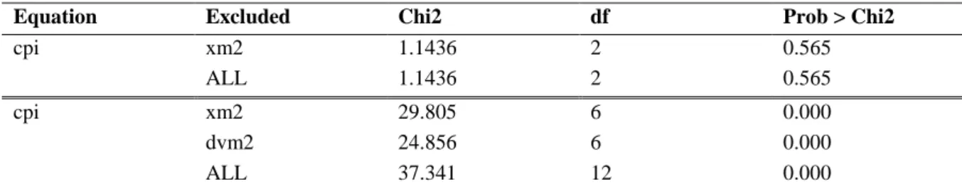
Money Supply Measures – Causality Study
After using the ADF test on CPI inflation rate, excess M2 growth and velocity of M2, it is
possible to see that the inflation rate and excess M2 growth are level stationary at the 5%
significance level, whereas velocity is difference stationary.
The long run causality from money to prices is well documented; it is the short run that incites
debate. Therefore, the interest lies in studying causality from money supply measures to
inflation in the shorter run, which is assessed using Granger causality tests after specifying the
data under a VAR model. The first relationship tested in this section is between CPI inflation
and excess M2 growth, following the traditional model derived from the equation of exchange.
Using the VAR lag selection procedure in STATA, all criteria indicate 2 as the number of
optimal lags. Next, the data is modeled and the Granger causality test is run, which does not
16 expected result given the qualitative analysis of the previous section regarding a disconnection
of money growth and prices.
However, when the equation is adjusted for the velocity of M2 – entering the model as first
difference to ensure stationarity – in an attempt to reflect effective money supply reaching the
real economy, and repeat the process above, the corresponding Granger test after a VAR (6)
shows strong causality, at the 1% significance level. This supports the hypothesis of a
connection between money supply and price level, as long as this relationship has an effective
impact on the real economy. Both of these specifications meet the stability, normality and no
autocorrelation criteria, tested using the eigenvalue, Jarque-Bera and Lagrange multiplier tests,
respectively.
Table 3 – Granger causality tests for money supply measures
Equation Excluded Chi2 df Prob > Chi2
cpi xm2 1.1436 2 0.565
ALL 1.1436 2 0.565
cpi xm2 29.805 6 0.000
dvm2 24.856 6 0.000
ALL 37.341 12 0.000
Notes: A probability below the 5% significance level means the null hypothesis of no Granger causality is rejected. Source: Author.
Real Activity Measures – Causality Study
Once more the ADF test is run, and out of the used variables, unemployment rate, average
hourly earnings growth, labor productivity, labor share, housing starts, total capacity utilization,
trade-weighted exchange rate and 10y-2y yield spread are first difference stationary, whereas
total compensation growth is level stationary.
Using a VAR model approach as above, and starting by testing the usual unemployment rate to
inflation relationship, an optimal lag length of 2 is selected by all criteria. Both significance and
17 that explores the transmission mechanism through wage growth, and a VAR with an optimal
lag of 6, no causality is found when using average hourly earnings, but the opposite happens
when using total hourly compensation, in a VAR (2) – confirming the hypothesis found in the
literature. In effect, using total compensation as a sole predictor rather than adding to the
unemployment rate leads to a better model taking into account the diagnosis tests for stability
and autocorrelation. In contrast, it is also demonstrated in this paper that adjusting for labor
share or productivity does not further improve the model. The hypothesis made is that total
compensation already reflects these two effects, as confirmed by running a Granger causality
test between these variables, which means productivity, labor share – and consequently, wage
inequality – are key drivers of inflation, albeit indirectly. These tests can be found in Table 4.
All specifications meet the criteria of no autocorrelation, normality and stability of the VAR
model.
Table 4 – Granger causality tests for real activity measures
Equation Excluded Chi2 df Prob > Chi2
cpi dunrate 13.354 2 0.001 ALL 13.354 2 0.001 cpi dahe 6.6069 6 0.359 ALL 6.6069 6 0.359 cpi comp 16.342 2 0.000 ALL 16.342 2 0.000 cpi comp 23.177 4 0.000 dlbsh 3.2624 4 0.515 dprod 1.5809 4 0.812 ALL 31.728 12 0.002 comp cpi 7.2425 4 0.124 dlbsh 36.881 4 0.000 dprod 32.693 4 0.000 ALL 64.005 12 0.000 Source: Author.
Numerous other activity measures have been used in the literature as augmented Phillips curve
models. Demonstrating the best results, according to Ang, Bekaert and Wei (2007), are
18 Capacity Utilization. After running Granger causality tests to each variable when added to the
best Phillips curve specification from above, it is demonstrated that Total Capacity Utilization
and the 10Y-2Y Yield Spread contribute the most to the model. When jointly added, these
variables are also shown to Granger cause inflation (Table 5). This gives support to the
hypothesis stipulated above that capacity utilization has a connection with inflation by putting
pressure on wages when at its peak, which then creates a pressure to increase price levels.
Furthermore, it also provides preliminary evidence that the yield curve slope is still a good
predictor, although a few peculiarities are presented later on this matter, regarding late sample
structural changes.
Table 5 – Granger causality tests for augmented Phillips curve specifications
Equation Excluded Chi2 df Prob > Chi2
cpi comp 9.8403 2 0.007 dhoust 1.3761 2 0.503 ALL 10.796 4 0.029 cpi comp 16.189 6 0.013 dtcu 20.274 6 0.002 ALL 38.548 12 0.000 cpi comp 4.8336 2 0.089 dtwfx 3.4532 2 0.178 ALL 9.742 4 0.045 cpi comp 8.1522 3 0.043 dspd 24.264 3 0.000 ALL 32.325 6 0.000 cpi comp 8.5071 3 0.037 dtcu 12.302 3 0.006 dspd 24.213 3 0.000 ALL 47.051 9 0.000 Source: Author.
Assessing Predictive Performance as Additional Support to Causality
In this section, forecasting models drawn from all conclusions made until this point are
proposed and tested against a common benchmark – the simple random-walk model where
19 defined throughout the previous section, we have: (a) – money supply model with excess M2
growth and velocity of M2 as predictors; (b) – the simple Phillips curve model with total
compensation growth as sole predictor; (c) – an augmented Phillips curve model which adds
total capacity utilization and the 10y-2y yield spread to the previous specification; and finally
(d) a joint model combining all predictors defined above. These models are estimated once
in-sample and then resulting coefficients are used to predict the expected year-on-year inflation
rate in the next quarter. For each model, this prediction is computed using estimations for the
equation corresponding to CPI inflation – the first out of the whole set of 𝑦1, … , 𝑦𝑚 dependent
variables that result from running a VAR (𝑝) model – as follows:
𝐸𝑡(𝑦1,𝑡+1) = 𝑐1+ 𝑎1,11 𝑦1,𝑡+ ⋯ + 𝑎11,𝑚𝑦𝑚,𝑡+ ⋯ + 𝑎1,1𝑝 𝑦1,𝑡−𝑝+1+ ⋯ + 𝑎1,𝑚𝑝 𝑦𝑚,𝑡−𝑝+1 (2)
where 𝑦1,𝑡+1 is the year-on-year inflation rate for quarter 𝑡 + 1, 𝑐1 is the estimated constant
term, 𝑎1,11 , … , 𝑎1,𝑚𝑝 are the estimated coefficients for each variable 1, … , 𝑚 at each lag 1, … , 𝑝
relative to the dependent variable 𝑦1, and 𝑦1,𝑡, … , 𝑦𝑚,𝑡−𝑝+1 are the variables 1, … , 𝑚 at each lag
1, … , 𝑝.
The criteria for in-sample to out-of-sample division was a simple 75%/25% rule, which gives
different out-of-sample periods for each model due to different sample sizes of the variables.
This is taken into account when comparing with the benchmark by using matching
out-of-sample periods between each model and the benchmark. Table 6 provides out-of-out-of-sample
calculations of the Relative Root Mean Squared Errors (RRMSE), meaning the ratios of each model’s RMSE divided by the benchmark’s RMSE. In Appendix 1 it is possible to verify the
stability of all these models and in Appendix 2 the normality and autocorrelation statistics.
According to Stock and Watson (2001) on VAR models, coefficients are typically not reported given the model’s complicated dynamics; Granger causality tests, for instance, are more
20 Overall, the models perform slightly better than the benchmark, giving support to the
conclusions drawn above on what fundamentally causes inflation. Regarding the diagnosis tests
of these models, no autocorrelation is found except on lags 2 and 3 of model (c) and on lag 4
of model (a). Normality is verified on all models except model (b). The implications are not
severe; non-normality is common in economic data and given the large sample size it should
not be a concern for Granger causality tests. With respect to autocorrelation, it could be argued
that it is an issue for model (c), however the test is highly sensitive to lag length and the criteria
used to choose an optimal lag length (AIC and BIC) do not aim to minimize autocorrelation –
which could mean overfitting the data – but rather to maximize predictive performance.
Table 6 – Out-of-Sample Performance
Model Out-of-Sample Period Relative to benchmark RMSE
(a) Money Supply VAR (6) 2004Q2:2018Q2 0.893
(b) Phillips Curve VAR (2) 2001Q1:2018Q2 1.034
(c) Augmented Phillips Curve VAR (3) 2008Q2:2018Q2 0.946
(d) Joint Model VAR (9) 2008Q4:2018Q2 0.941
Source: Author.
Discussion and Closing Remarks
In the section above, various Granger causality tests were run following theoretical and
empirical based specifications, under a VAR modeling approach. These tests provide evidence
that inflation in the US is determined by its own lags, excess M2 growth, the velocity of M2,
total compensation growth, total capacity utilization and the 10Y-2Y Yield Spread, which is
also supported by good predictive performance out-of-sample. Although it is recognized that
the models might exhibit biases, in general, the diagnosis tests support the models and the good
out-of-sample performance using different samples for each, indicate a solid empirical result.
These results show an improvement over their respective traditional specifications – either
21 core hypothesis here presented was that inflation, as a very complex and non-linear process,
can hardly be modeled by the same approach as structural changes happen in the economy that
fundamentally change the way traditional transmission mechanisms affect prices. It is crucial
that asset managers understand what drives inflation through structural changes, and for that it
is necessary to understand what impact these changes have and how to correct the relationships
accordingly. This paper has shown the main changes in the US inflationary process in the last
decades:
An imbalance in the money to prices connection resulting from a greater dominance of
flows to the financial system that are not allocated to real investment and transactions,
and, recently, a combination of tighter credit restrictions, slowly recovering balance
sheets and central bank incentives that caused banks to keep unprecedented levels of
excess reserves;
A low labor productivity economy which, aggravated by wage inequality and lower
labor share of income, disconnects output growth to price growth even for short term
horizons.
These are symptomatic of highly developed economies, and as such, moderation in economic
variables including inflation is likely to remain in the near future.
Additionally, it was demonstrated that total capacity utilization contributes to inflation by
intensifying the transmission mechanism from activity measures to prices and that the yield
spread is a good predictor. On the latter, a few remarks are in order. Causality tests are run for
the whole sample in this paper, and therefore, some positive bias can exist, mitigating late
sample structural changes. Such is the case for the yield curve slope; recently, while the spread
has decreased significantly, it has to be noted that the Fed had been offering assets across
22 more of a structural construct rather than a reflection of expectations, at least until a reversal to
conventional monetary policy.
Going forward, a few aspects are of major relevance for asset managers with respect to the US.
The effect of reversing quantitative easing and, more importantly, excess reserves, must be
carefully monitored due to its lack of comparable precedents. A few undesirable scenarios could
take place; the Fed is likely to raise interest rates, ease credit restrictions and reduce incentives
on holding reserves very gradually in order to prevent excessive inflationary pressures,
however, a sudden growth spur might incentivize banks to loan their readily accessible reserves,
leaving the Fed with little or no timing to react. On the other hand, an economic downturn
during this slow transition period would leave little room for the Fed to reduce rates if at that
time they are still low. The productivity landscape will also be crucial, especially being a
developed country such as the US. Since GDP growth is driven by two factors: productivity
and labor hours/numbers, and given a decreasing weight of labor hours and workers on GDP
growth, as seen in the labor market trends discussed previously, productivity becomes the core
driver of GDP growth. As such, private investment in human capital and tangible assets are key
drivers to monitor in order to assess the economy’s ability to continue growing. These have
shown an unimpressive trend in recent years.
Having screened through the major influences on inflation, this paper is concluded. It has demonstrated the importance of adjusting inflation’s core drivers to structural changes,
23
Appendices
Appendix 1 – VAR Stability Tests
Notes: Eigenvalues below 1, i.e. within the circle, indicate VAR stability. Source: Author.
Appendix 2 – VAR Autocorrelation and Normality Tests
Probability > Chi2 LM Autocorrelation Test
per Lag
Model (a) Model (b) Model (c) Model (d)
1 0.825 0.202 0.288 0.287 2 0.183 0.746 0.002 0.330 3 0.321 - 0.000 0.264 4 0.000 - - 0.985 5 0.217 - - 0.392 6 0.143 - - 0.395 7 - - - 0.513 8 - - - 0.599 9 - - - 0.135
Jarque-Bera Normality Test 0.854 0.000 0.356 0.549
Notes: Probabilities below the 5% significance level mean the null hypothesis of normality/no autocorrelation is rejected. Source: Author. -1 -. 5 0 .5 1 Ima g in a ry -1 -.5 0 .5 1 Real Roots of the companion matrix
-1 -. 5 0 .5 1 Ima g in a ry -1 -.5 0 .5 1 Real Roots of the companion matrix
-1 -. 5 0 .5 1 Ima g in a ry -1 -.5 0 .5 1 Real Roots of the companion matrix
-1 -. 5 0 .5 1 Ima g in a ry -1 -.5 0 .5 1 Real Roots of the companion matrix
(a) (b)
24
References
Anderson, R.G., 2007. “How well do wages follow productivity growth?” Economic
Synopses, No. 7.
Ang, A., Bekaert, G. and Wei, M., 2007. “Do macro variables, asset markets, or surveys
forecast inflation better?” Journal of Monetary Economics, 54 (2007): 1163–1212.
Assenmacher-Wesche, K. and Gerlach, S. 2008a. “Money growth, output gaps and
inflation at low and high frequency: Spectral estimates for Switzerland.” Journal of
Economic Dynamics and Control, vol. 32 (2): 411-435.
Assenmacher-Wesche, K. and Gerlach, S., 2008b. “Interpreting euro area inflation at
high and low frequencies,” European Economic Review, vol. 52 (6): 964-986.
Atkeson, A. and Ohanian, L.E., 2001. “Are Phillips curves useful for forecasting
inflation?” Federal Reserve Bank of Minneapolis Quarterly Review, 25: 2–11.
Azevedo, J.V. and Pereira, A., 2010. “Forecasting inflation with monetary aggregates.”
Economic Bulletin, Banco de Portugal, vol. 16 (3): 151-168.
Benkovskis, K., Caivano, A.M., et al. 2011. “Assessing the sensitivity of inflation to
economic activity.” Working Paper Series, No. 1357.
Binner, J.M., et al., 2009. “Does Money Matter in Inflation Forecasting?” Federal
Reserve Bank of St. Louis Working Paper, 2009-030B.
Blanchard, O., Cerutti, E. and Summers, L., 2015. “Inflation and Activity - Two
Explorations and their Monetary Policy Implications.” NBER Working Paper, No.
21726.
Friedman, Milton. 1963. “Inflation: Causes and Consequences.” New York: Asia
Publishing House.
Gordon, Robert J., 1988. “Modern theories of inflation.” In Macroeconomics: Theory
25 Inoue, A. and Kilian, L., 2008. “How Useful is Bagging in Forecasting Economic Time
Series? A Case Study of U.S. CPI Inflation” Journal of the American Statistical
Association, vol. 103 (482): 511-522.
Koop, G. and Korobilis, D., 2009. “Forecasting Inflation Using Dynamic Model
Averaging” Rimini Center for Economic Analysis, WP 34-09.
Lanne, M., Luoto, J. and Nyberg, H., 2014. “Is the Quantity Theory of Money Useful
in Forecasting U.S. Inflation?” CREATES Research Paper, No. 26.
Phillips, A.W., 1958. “The Relation Between Unemployment and the Rate of Change
of Money Wage Rates in the United Kingdom, 1861-1957.” Economica, New Series,
vol. 25 (100): 283-299
Quévat, B. and Vignolles, B., 2018. “The relationships between inflation, wages and
unemployment have not disappeared.” Conjoncture in France, March 2018: 19-34. Schwellnus, C., Kappeler, A. and Pionnier, P. 2017. “Decoupling of wages from
productivity: Macro-level facts.” OECD Economics Department Working Papers, No.
1373. Paris: OECD Publishing.
Smets, F. and Wouters, R., 2007. “Shocks and Frictions in US Business Cycles: A
Bayesian DSGE Approach.” American Economic Review, vol. 97 (3): 586-606. Stock, J.H., and Watson, M.W., 1999. “Forecasting inflation.” Journal of Monetary
Economics, vol. 44 (1999): 293-335.
Stock, J.H. and Watson, M.W., 2001. “Vector Autoregressions.” Journal of Economic
Perspectives, vol. 15 (4): 101-115.
Stock, J.H. and Watson, M.W., 2008. “Phillips Curve Inflation Forecasts.” NBER
Working Paper, No. 14322.
Woodford, M., 2007a. “How Important is Money in the Conduct of Monetary Policy?”