Analysis of European Countries’ Vulnerabilities through
Statis Methodology
by
Catarina Lourenço Soares
Dissertation for the degree of Master in Economics
Porto School of Economics
Dissertation supervised by:
Professora Doutora Adelaide Maria de Sousa Figueiredo
Professora Doutora Fernanda Otília de Sousa Figueiredo
ii
B
IOGRAPHICAL
N
OTE
Catarina Lourenço Soares was born on 25th of August 1990 and is a native of Pedroso, municipality of Vila Nova de Gaia, Oporto district. She finished the secondary school in the scientific-technical course of account management, economics field, in Colégio Internato dos Carvalhos. However, the feeling that her journey was not finished together with a willingness to learn and improve her skills, made her join the Porto School of Economics in the degree of economics, without truly knowing specifically what an economist was. She graduated in Economics, in 2011, and with a passion for this area, joined the Master’s Degree of Economics in the specialization of Economic Analysis.
She has complemented her higher education with other activities no less important to her personal development. She is fluent in English and has knowledge of Spanish. But as in these languages only the words change, she embraced another challenge - Mandarin, not for professional reasons but for the sheer challenge. Currently, she is taking an internship at Deutsche Bank and teaches Maths and English tutorials.
This dissertation represents the conclusion of one more stage of my life with a sense of mission accomplished…
iii
A
CKNOWLEDGEMENTS
Firstly, I want to thank to my supervisors Prof. Adelaide Figueiredo and Prof. Fernanda Figueiredo for their support, availability, suggestions and ideas, which were very important to the realization of this dissertation.
I express my special thanks to my family for giving me wings to grab every opportunity that have been coming and for being there, in the happy and difficult moments, to support me and to share a great part of my life.
I want to thank to all my friends and, in special, to Magui, Carla and Mónica. Magui for being my company throughout “the difficult ways”, for their friendship and camaraderie. To Carla, a long-time friend, for knowing me so well. To Mónica for her motivating words and strange adventures.
iv
A
BSTRACT
The subprime crisis, originated in the United States of America in August 2007, quickly became a global financial crisis, affecting a large number of countries, including mainly the European economies. Europe also faces a crisis of public debt, particularly since the beginning of 2010, having the Greek debt served as a "fuse".
In this economic context, it becomes imperative to identify, analyse and discuss the main economic weaknesses that contribute to the widely and differentially smite of the European countries.
In this sequence, this study aims to know which the main vulnerabilities of these countries are and what conclusions can be drawn. For this purpose, inspired by the early warning systems, thirty-one variables are analysed through the Statis methodology. This methodology allows us to analyse simultaneously multiple data tables, determining a common structure among the European countries.
Accordingly, we concluded that the years 2002-2004, 2006-2007 and 2009-2011 have, in general, been identified as the most similar, seeming the year of 2008 to be a "turning point" between them. In this sense, the Statis methodology highlighted the economic developments in the period 2002-2011 and allowed to obtain interesting conclusions about what have twenty-seven European countries in common, after all, and what differentiate them to each other.
v
C
ONTENTS BIOGRAPHICAL NOTE ... ii ACKNOWLEDGEMENTS ... iii ABSTRACT ... iv PREFACE ... 1 CHAPTER 1 ... 2The Recent Global Financial Crisis and Some Considerations About EWS ... 2
1.1 The recent financial crisis ... 2
1.1.1 From the U.S. subprime crisis to the global crisis ... 3
1.1.2 The response of economic policy ... 6
1.1.3 This crises’ similarities with previous crisis and among countries involved ... 9
1.2 Early warning systems: goals, structure and evolution ... 11
1.2.1 The essence and evolution of Early Warning Systems ... 11
1.2.2 Some considerations in the development of an Early Warning System ... 13
1.2.3 Limitations and the need for future developments ... 16
CHAPTER 2 ... 18
Methodology and Description of the Data ... 18
2.1 Statis methodology ... 18
2.2 Variables and countries analysed ... 20
2.3 Previous data treatment ... 23
2.4 Preliminary analysis of the data set ... 24
CHAPTER 3 ... 31
Macroeconomic Variables ... 31
3.1 Conclusions of the Statis method ... 31
Interstructure ... 31
Intrastructure ... 33
Contribution of the countries to the differences between years and their trajectories36 3.2 Results of the Dual Statis method ... 40
Interstructure ... 40
Intrastructure ... 41
Contribution of the variables to the difference between years and their trajectories43 CHAPTER 4 ... 45
Competitiveness and External Debt ... 45
4.1 Competitiveness ... 45
4.1.1 Conclusions of the Statis method ... 45
vi
Intrastructure ... 47
Countries’ contribution to the differences between years and their trajectories ... 49
4.1.2 Results of the Dual Statis method ... 52
Interstructure ... 52
Intrastructure ... 53
Contribution of the variables to the differences between years and their trajectories54 4.2 External Debt ... 56
4.2.1 Conclusions of the Statis method ... 56
Interstructure ... 56
Intrastructure ... 57
Contribution of the countries to the differences between years and their trajectories60 4.2.2 Results of the Dual Statis method ... 63
Interstructure ... 63
Intrastructure ... 64
Contribution of the variables to the differences between years and their trajectories65 CHAPTER 5 ... 67
Public, Private and Financial Sectors ... 67
5.1 Public Sector ... 67
5.1.1 Conclusions of the Statis method ... 67
Interstructure ... 67
Intrastructure ... 69
Contribution of the countries to the differences between years and their trajectories72 5.1.2 Results of the Dual Statis method ... 75
Interstructure ... 75
Intrastructure ... 76
Contribution of the variables to the differences between years and their trajectories78 5.2 Private and Financial Sectors ... 80
5.2.1 Conclusions of the Statis method ... 80
Interstructure ... 80
Intrastructure ... 81
Contribution of the countries to the differences between years and their trajectories84 5.2.2 Results of the Dual Statis method ... 87
Interstructure ... 87
Intrastructure ... 88
Contribution of the variables to the differences between years and their trajectories90 CHAPTER 6 ... 92
Concluding Remarks ... 92
vii
APPENDIX ... 102
Appendix 1 – Variables. ... 102
Appendix 2 – Boxplots of the variables. ... 105
viii
Tables
Table 2.1 - Macroeconomic variables considered in the study. ... 21
Table 2.2 - Variables that feature the public sector. ... 22
Table 2.3- Group of variables of country's competitiveness. ... 22
Table 2.4 - Group of variables of external debt. ... 22
Table 2.5 - Private and financial sectors’ variables. ... 23
Table 2.6 - Average of the variables. ... 24
Table 2.7- Median, maximum and minimum values of the variables. ... 25
Table 2.8 - Fisher skewness coefficients. ... 26
Table 2.9 - Kurtosis coefficients. ... 27
Table 2.10 - Linear correlation coefficients among macroeconomic variables in 2002. 27 Table 2.11 - Linear correlation coefficients among macroeconomic variables in 2011. 27 Table 2.12 - Linear correlation coefficients of the public state's variables in 2002. ... 28
Table 2.13 - Linear correlation coefficients of the public state's variables in 2011. ... 28
Table 2.14 - Linear correlation coefficients of the competitiveness' variables in 2002. 29 Table 2.15 - Linear correlation coefficients of the competitiveness' variables in 2011. 29 Table 2.16 - Linear correlation coefficients of the external debt' variables in 2002 (left) and 2011 (right). ... 29
Table 2.17 - Linear correlation coefficients of the private and financial sectors' variables in 2002 (left) and 2011 (right). ... 30
Table 3.1 - Matrices of the RV coefficients (above) and Hilbert-Schmidt distances (below). ... 32
Table 3.2 – Scalar products and distances among data tables’ representative objects and the compromise object. ... 33
Table 3.3 – Eigenvalues, inertia and cumulative inertia of the first eight axes. ... 33
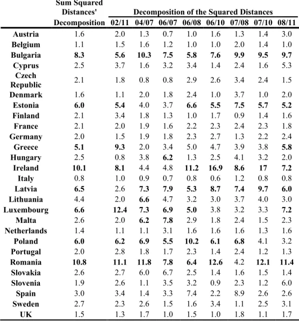
Table 3.4 – Decomposition of the sum of squared distances and decomposition of the squared distances into percentage of individuals’ contributions. ... 38
Table 3.5 - Matrix of the distances between years’ representative objects. ... 40
Table 3.6 – Scalar products and distances among data tables’ representative objects and the compromise object. ... 41
ix Table 3.7 – Eigenvalue, inertia and cumulative inertia of the first eight compromise axes. ... 41 Table 3.8 – Sum square distances’ decomposition and squared distances’ decomposition into percentage of variables’ contribution. ... 44 Table 4.1 - RV coefficients (above) and distances (below) between data tables'
representative objects. ... 46 Table 4.2 - Scalar products and distances among the compromise object and data tables' representative objects. ... 47 Table 4.3 - Distances between data tables' representative objects. ... 52 Table 4.4 - Scalar products and distances between the compromise object and data tables' representative objects. ... 53 Table 4.5 - RV coefficients (above) and distances (below) between data tables'
representative objects. ... 56 Table 4.6 - Scalar products and distances among different data tables. ... 57 Table 4.7 - Distances between correlation matrices. ... 63 Table 4.8- Scalar products and distances among the compromise object and data tables' correlation matrices. ... 64 Table 5.1 – RV coefficients (above) and distances (below) between data tables’
representative objects. ... 68 Table 5.2 – Scalar products and distances among data tables’ representative objects and the compromise object. ... 69 Table 5.3 - Distances between representative objects. ... 75 Table 5.4 - Scalar products and distances among the compromise object and data tables' representative objects. ... 76 Table 5.5 - Scalar products (above) and distances (below) among data tables'
representative objects. ... 80 Table 5.6 - Scalar products and distances among compromise object and data frames' representative objects. ... 82 Table 5.7 - Distances between data tables' representative objects. ... 87 Table 5.8 - Scalar products and distances among the compromise object and correlation matrices. ... 88
x Table A.1 - Variables: source and description. ... 102 Table A.2 – Linear correlation coefficients between macroeconomic variables and each compromise axis (1, 2, 3 and 4). ... 108 Table A.3 – Linear correlation coefficients between competitiveness' variables and compromise axes (1, 2 and 3). ... 109 Table A.4 – Linear correlation coefficients between debt's variables and compromise axes (1, 2, 3, and 4). ... 110 Table A.5 – Linear correlation coefficients between private and financial sectors' variables and compromise axes (1, 2, 3, 4 and 5). ... 111 Table A.6 – Linear correlation coefficients between public sector’s variables and compromise axes (1, 2, 3 and 4). ... 112
xi
F
igures
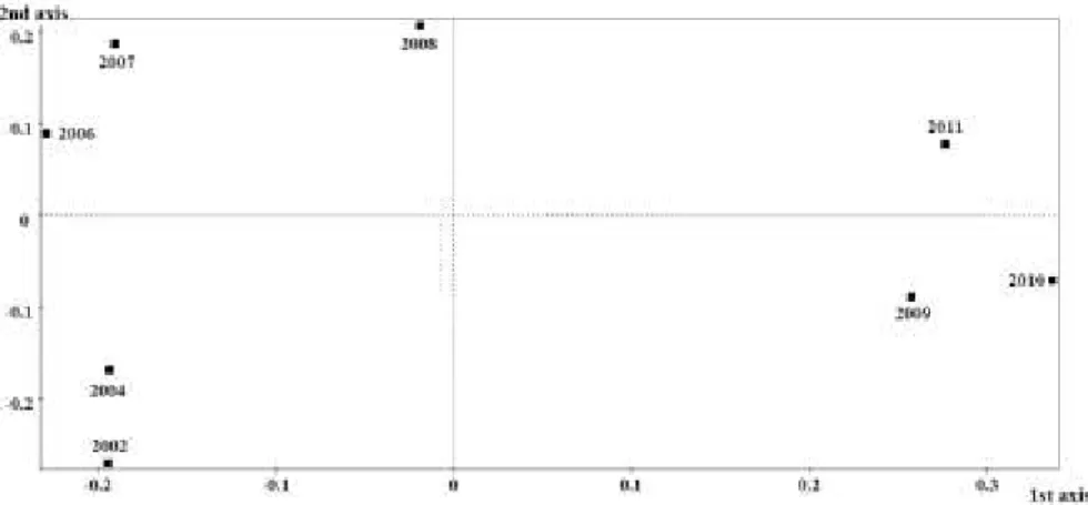
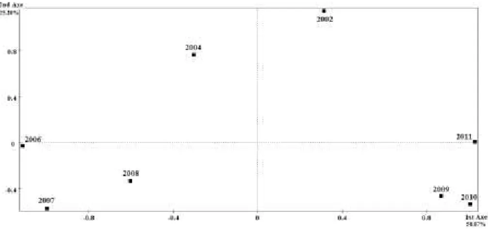
Figure 3.1 – Centred Interstructure Euclidean Image in the plan [1, 2]. ... 33
Figure 3.2 – Compromise’s Euclidean Image in the plan [1, 2]. ... 34
Figure 3.3 - Compromise’s Euclidean Image in the plan [1, 3]. ... 35
Figure 3.4 - Compromise’s Euclidean Image in the plan [1, 4]. ... 36
Figure 3.5 – Countries’ trajectories in the plan [1, 2]. ... 39
Figure 3.6 - Centred Interstructure Euclidean Image in the plan [1, 2]. ... 41
Figure 3.7 - Compromise’s Euclidean Image in the plan [1, 2]. ... 42
Figure 3.8 - Compromise’s Euclidean Image in the plan [1, 3]. ... 42
Figure 3.9 - Compromise’s Euclidean Image in the plan [1, 4]. ... 43
Figure 3.10 - Trajectories of each variable in the plan [1, 2]. ... 44
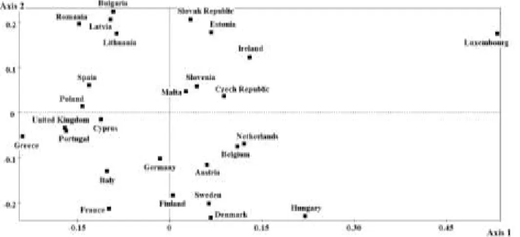
Figure 4.1 - Centred Interstructure Euclidean Image in the plan [1, 2]. ... 46
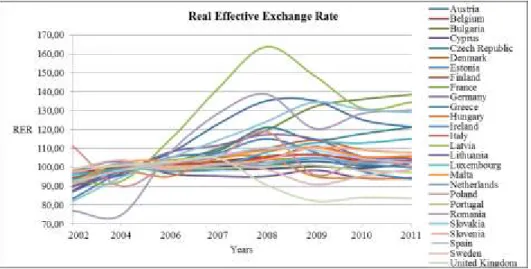
Figure 4.2 – Real effective exchange rate of the European countries. ... 47
Figure 4.3 - Compromise’s Euclidean Image in the plan [1, 2]. ... 48
Figure 4.4 - Compromise’s Euclidean Image in the plan [1, 3]. ... 49
Figure 4.5 - Countries' trajectories in the plan [1, 2]. ... 51
Figure 4.6 - Centred Interstructure Euclidean Image in the plan [1, 2]. ... 53
Figure 4.7- Compromise’s Euclidean Image in the plan [1, 2]. ... 53
Figure 4.8 - Compromise’s Euclidean Image in the plan [1, 3]. ... 54
Figure 4.9 - Each variable trajectory in the plan [1, 2]. ... 55
Figure 4.10 - Centred Interstructure Euclidean Image in the plan [1, 2]. ... 57
Figure 4.11 - Compromise’s Euclidean Image in the plan [1, 2]. ... 58
Figure 4.12 - Compromise’s Euclidean Image in the plan [1, 3]. ... 59
Figure 4.13 - Compromise’s Euclidean Image in the plan [1, 4]. ... 59
Figure 4.14 - Countries' trajectories defined in the plan [1, 2]. ... 62
Figure 4.15 - Centred Interstructure Euclidean Image in the plan [1, 2]. ... 63
Figure 4.16 - Compromise’s Euclidean Image in the plan [1, 2]. ... 64
Figure 4.17 - Compromise’s Euclidean Image in the plan [1, 3]. ... 65
Figure 4.18 - Compromise’s Euclidean Image in the plan [1, 4]. ... 65
Figure 4.19 - Variables' trajectories in the plan [1, 2]. ... 66
xii
Figure 5.2 - Compromise’s Euclidean Image in the plan [1, 2]. ... 69
Figure 5.3 - Compromise’s Euclidean Image in the plan [1, 3]. ... 70
Figure 5.4 - Compromise’s Euclidean Image in the plan [1, 4]. ... 71
Figure 5.5 - Trajectories of each country in the plan [1, 2]. ... 74
Figure 5.6 - Centred Interstructure Euclidean Image in the plan [1, 2]. ... 76
Figure 5.7 - Compromise’s Euclidean Image in the plan [1, 2]. ... 76
Figure 5.8 - Compromise’s Euclidean Image in the plan [1, 3]. ... 77
Figure 5.9 - Compromise’s Euclidean Image in the plan [1, 4]. ... 78
Figure 5.10 - Variables’ trajectories in the plan [1, 2]. ... 79
Figure 5.11 - Centred Interstructure Euclidean Image in the plan [1, 2]. ... 81
Figure 5.12 - Compromise’s Euclidean Image in the plan [1, 2]. ... 82
Figure 5.13 - Compromise’s Euclidean Image in the plan [1, 3]. ... 83
Figure 5.14 - Compromise’s Euclidean Image in the plan [1, 4]. ... 83
Figure 5.15 - Compromise’s Euclidean Image in the plan [1, 5]. ... 84
Figure 5.16 - Countries’ trajectories defined in the plan [1, 2]. ... 86
Figure 5.17 - Centred Interstructure Euclidean Image in the plan [1, 2]. ... 87
Figure 5.18 - Compromise’s Euclidean Image in the plan [1, 2]. ... 89
Figure 5.19 - Compromise’s Euclidean Image in the plan [1, 3]. ... 89
Figure 5.20 - Compromise’s Euclidean Image in the plan [1, 4]. ... 90
Figure 5.21 - Trajectories of the variables in the plan [1, 2]. ... 91
Figure A.1 - Boxplots of the variables in 2002 and 2011, respectively. ... 105
Figure A.1 - Boxplots of the variables in 2002 and 2011, respectively (cont.). ... 106
1
P
REFACEIssing (2011), page 6, states that "(...) the crisis was anything but a surprise when
it arrived, it was, so to speak, a "crisis foretold"." In this sequence, which
vulnerabilities do the countries of the European Union, the largest economic and political union in the world, have in their economies? What have these countries of similar and different? What binds twenty-seven different economies? Why is the present global financial crisis affecting them so differently? Due to its actuality and scientific relevance, this study focuses on this issue.
Therefore, through the analysis of the vulnerability indicators present in early warning systems, which are intended to predict the occurrence of a crisis in a certain time horizon, we want to know which the main vulnerabilities of European countries are and what conclusions can be drawn. For this purpose, a methodology of conjoint analysis of data tables is used – the Statis methodology - introduced in L'Hermier des Plantes (1976) and later developed by Lavit (1988) and Lavit et al. (1994). This methodology allows to analyze simultaneously multiple data frames, determining a common structure between individuals and/or observed variables.
Subsequently, Chapter 1 is about the recent global financial crisis. It also provides a brief description of the response given by the economic policy, the similarities that can be found with previous crises as well as between the U.S. economy and European countries’ economies. In the end, this chapter focuses on the early warning systems, models that inspired this thesis. Here is made a small description of their goals and developments.
Chapter 2 begins with a brief reference to Principal Components Analysis methodology which is the basis methodology of the Statis. Then the Statis methodology is described along with a presentation of the data here used and a preliminary analysis of it.
The chapters 3, 4 and 5 exploit the conclusions that can be drawn by the application of Statis and Dual Statis methods to variables collected for the twenty-seven European countries during the period 2002- 2011, and which feature macroeconomics, public sector, competitiveness, debt and, financial and private sector, respectively. Chapter 6 concludes.
2
C
HAPTER
1
The Recent Global Financial Crisis and Some Considerations
About Early Warning Systems
1.1 The recent financial crisis
The recent financial crisis, the first global financial crisis since the Great Depression in 1929 (Claessens et al., 2010) and now considered the most harmful since it1, is in the words of Rose et al. (2012, pg. 3) "notable for a number of reasons including, most
obviously, its severity and speed". Thus, the subprime crisis started in the U.S. in 2007,
quickly became a global crisis, leading to a worldwide recession (Bordo et al., 2010). Schwartz (1987) warned that the origin of a financial crisis is a banking crisis and this crisis is not an exception (Bordo et al., 2010).
Global growth, stable inflation, productivity growth and low interest rates; it was, according to the International Monetary Fund (IMF, 2009), the world economic context in the years preceding the crisis. However, fairy tales do not exist in real life, and therefore, the high global growth obscured what is called as global imbalances. The current account surpluses of the Asian countries (especially China and oil-exporting countries) triggered a US’ current account deficit (Eichengreen, 2004; Reinhart et al., 2008b and Diamond et al., 2009) and contributed to low interest rates (IMF 2009).
The high demand in the U.S. led to the creation of new financial instruments riskier than what was expected (IMF, 2009), contributing to a greater fragility of the financial system. Some of these instruments were used to finance the bubble in real estate and were acquired by investment banks and other financial institutions, against short-term debt. This is considered one of the main causes of the crisis (Diamond et al.,
1 Studies such as Bordo et al. (2010) report the Great Depression as the worst crisis happened so far,
getting the recent financial crisis in the second place. It is, however, worth stressing that some studies may have truncate errors, due to effects of the recent crisis in the years following the year of the study.
3 2009). However, Rose et al. (2012) argue that the weak regulation was not only present in the securitization and indicates the poor financial regulation, not only in U.S., but also internationally. This is also advocated by IMF (2009) which adds failures in macroeconomic policies and a dispersed supervision.
But how has the recent financial crisis developed?
1.1 .1 From the U.S. subprime crisis to the global crisis
In the US, in the years preceding the crisis, there was a sharp increase in house prices and other asset markets, especially in stock market (Reinhart et al., 2008b and Rose et
al., 2012). This was triggered by expansionary monetary policy conducted by the
Federal Reserve and other incentives from the government to house purchase (Reinhart
et al., 2008b; Diamond et al., 2009 and Bordo et al., 2010).
These booms in real estate and stock market were also associated to the fast credit growth (Claessens et al., 2010), as in previous crises (Reinhart et al., 2008b), but this time concentrated in a market: the subprime (Claessens et al., 2010). The mortgage market was very dependent on the houses’ prices, as they serve as a collateral asset, giving the capital needed to pay the loan by its owner, serving as guarantee (Claessens
et al., 2010 and Diamond et al., 2009). However, these mortgages were also granted to
subprime borrowers, i.e., borrowers with low means of payment, creating investment portfolios very exposed to a price decline (Claessens et al., 2010).
The increase in credit and the innovation generated by the financial sector contributed to an increase in household debt, particularly after 2000 (Claessens et al., 2010). This made them vulnerable to macroeconomic conditions, as the slowdown in economic activity, decline in house prices and changes in credit conditions, and was responsible for the transmission of the crisis from the financial sector to the real sector, hampering the response of the political authorities (Claessens et al., 2010).
The securitization and creation of new financial instruments allowed a credit expansion, but had also increased the fragility of the financial sector, since it contributed to the lack of transparency (Buiter, 2007) and liquidity once house prices began to decline (Claessens et al., 2010). The demand of securities with AAA rating by international investors had propitiated that, with the use of securitization, mortgages could have started to be transacted in the market, making them net (Mortgage-backed
4 securities - MBS). Thereby, they were transacted with other mortgages from other areas and began to give rise to other instruments, which could subsequently be separated and traded with others (Diamond et al., 2009). Many of these new instruments, such as Asset-Backed Securities (ABS), Collateralized Mortgage Obligations (CMO), Collateralized Loan Obligation (CLO) or Collateralized Debt Obligation (CDO), were evaluated with AAA rating (Diamond et al., 2009 and Claessens et al., 2010). The use of securitization and the use of the "originate to distribute" generated agency problems, bringing consequences for final consumers and increasing systemic risk.
This was exacerbated by the gap shown in the rating process. These agencies assessed the instruments based only on the general information collected, ignoring other detailed information about the solvency and credibility, fomenting weak monitoring of the debtors, and giving an underestimation of the financial products’ risk (Diamond et
al., 2009 and Claessens et al., 2010). Other justifications for the poor assessment, as
overconfidence by the rating agencies in relation to their own abilities (Coval et al., 2009) or conflicts of interest (IMF, 2009), are likely to be found in the literature.
The credit boom had also provided another consequence. Transactions which arise out of the banking regulations had also started to grow. The so-called "shadow banking
system" was comprised by investment banks, hedge funds, money market funds,
mortgage lenders and other financial institutions and acted out of banking regulation2 and without the necessary supervision, contributing to the increase in systemic risk (IMF, 2009), but giving high profits (Claessens et al., 2010).
In the summer 2007, due in part to a contraction in monetary policy, interest rates rose and house prices began to decline, causing defaults especially in subprime or near-prime mortgages (Reinhart et al., 2008b; Claessens et al. 2010 and Rose et al., 2012). The complexity of these new instruments, besides affecting the liquidity of the market and reducing the securitization, combined with a lack of transparency in the balance sheets of financial institutions, led to adverse selection problems, given the difficulty in recognizing which institutions were "healthy" (Claessens et al., 2010). This was transmitted to other financial and real estate markets in the U.S. and affected the
2 Different types of financial institutions were regulated differently. Thus, opportunities for regulatory
arbitrage had been exploited by the shadow banking system, leading to highly leveraged institutions (IMF, 2009).
5 interbank market, particularly after August 2007 (Lenza et al., 2010). Additionally, it had a negative effect on consumption, given the leverage of households and the contraction in credit, leading to a decrease in activity and profits of the business sector, rising unemployment, more mortgage defaults and the slowdown of economic activity (Claessens et al., 2010).
The transmission to other countries was boosted by financial integration. As Claessens et al. (2010) pointed out, not only had financial integration increased the efficiency and international risk sharing, but it had also eased contagion of international financial shocks. The instruments originated in the U.S. were owned by private investors, institutional and public sectors of many countries, since it seemed to have an attractive combination between risk, returns and liquidity (Claessens et al., 2010 and Rose et al., 2010). In particular to the financial sector, these instruments were very attractive given their profitability, despite their risk3. However, since they were new financial instruments, it was difficult to assess whether the profitability offered was excessive given their risk or a premium by inherent risk (Diamond et al., 2009).
The first phase of crisis’ transmission was through these direct exposures, causing problems in the U.S. financial system and starting to spread to the European’s, evidenced by the problems faced in Germany (IKB in July 2007) and France (BNP Paribas in August 2007) (Claessens et al., 2010 and Rose et al., 2010). The leverage in the financial sector, both in U.S. and in Europe, limited it to absorb losses and provoked a decline in confidence and the increase of risk between counterparties (Claessens et al., 2010 and Rose et al., 2010). Additionally, the credit deterioration caused ratings’ declines (Claessens et al., 2010).
The second phase of the crisis’ transmission was through the asset market (Claessens et al., 2010). Leveraged financial institutions and with losses due to the decline in the price of ABS, resorted to the market in order to obtain funds, generating liquidity shortages (Davis, 2008 and Claessens et al., 2010), the freezing of the capital markets, further decline in stock prices and exchange rate fluctuations, leading to a
3 Other reasons were also pointed in the literature for the high demand of these new instruments, despite
their risk. Among them, the incentive systems (evaluation of CEOs in accordance with annual profits), internal control and compensation systems (especially in the case of traders), which led to excessive risk taking by traders and managers in order to take advantage of the profitability’s differential between the new instruments and other AAA assets (Diamond et al., 2009 and IMF, 2009). Rose et al. (2012) and Buiter (2009) also suggest the lack of ethical, moral and quality governance in institutions.
6 sharp drop in confidence (Claessens et al., 2010). In the summer of 2008 as referred in Mishkin (2011, pg. 5), the crisis seemed to be controlled, since "the subprime sector
constituted only a small part of the capital market and the losses in MBS, although substantial, appeared to be managed”. On 15th September 2008, the fourth largest U.S.
investment bank - Lehman Brothers - declared bankruptcy, due to subprime market’s exposure (Mishkin, 2011), giving a systemic dimension to the crisis.
The third phase of the crisis’ transmission was due to concerns about solvency after this event (Claessens et al., 2010). Mishkin (2011) and Lenza et al. (2010) pointed the near collapse of AIG on 16 September 2008, the pursuit of the Reserve Primary Fund on the same day and the difficulties in approving the Trouble Asset Relief Plan (TARP) in the U.S., as causes that, in addition to the bankruptcy of Lehman Brothers, had increased turbulence in financial markets and turned the subprime crisis global.
These events highlighted the excessive risk taking, the fragility and lack of transparency of the financial system (Mishkin, 2011). The high losses of financial institutions, forced them to deleverage, increasing the sale of assets, encouraging more asset price declines and the need for recapitalizations (Claessens et al., 2010). Heightened the tensions in financial markets, mainly in money market (Lenza et al., 2010), the spreads of interest rates of the euro, dollar and pound sterling rose to historic levels (Lenza et al., 2010 and Mishkin, 2011) and confidence has globally reduced dramatically (Claessens et al., 2010).
The crisis also spread through the real channel. As Bordo et al. (2010, pg. 4) highlighted "international crises are inevitably associated with recessions". Enhanced by the decline in demand in many advanced economies, given the recession in these countries, and the deterioration of international trade, exports declined, leading to a worldwide recession (Claessens et al., 2010 and Bordo et al., 2010).
1.1.2
The response of economic policy
Different monetary policy instruments were used by Central Banks in response to the economic recession which has arisen, especially, after the collapse of Lehman Brothers, including standard and non-standard measures (Lenza et al., 2010). In some periods it was also possible to find concerted actions between them. Some of these measures are highlighted below.
7 Before Lehman Brothers’ bankruptcy, the authorities clashed with problems as the reduction of confidence, increase in risk aversion and difficulties in obtaining liquidity. Thus, the interventions of the European Central Bank (ECB), the Federal Reserve and the Bank of England, aimed to provide liquidity to the banking sector and to support banking intermediation in the money market (Lenza et al., 2010). The ECB allowed the Euro Area’ banks to mobilize the amount of liquidity required and conducted additional refinancing operations (Lenza et al., 2010), even though continuing to pursue its strategy of inflation targeting (Eichengreen, 2012). The Bank of England increased the list of eligible assets, including ABS, and the maturity of some operations. Additionally, it launched the Special Liquidity Scheme, which allowed a swap between illiquid assets for Treasury Bills up to three years. The Federal Reserve provided additional liquidity through its normal operations and increased the maturity of discount window operations. It also launched unconventional measures, such as the development of the Term Auction Facility (TAF) and the possibility of purchasing Treasury Securities with illiquid assets as collateral. Additionally, some financial institutions had to be rescued, as Bear Stearns which failed to have access to short-term financing or in converting their long-term assets at a fair price, and was bought by JP Morgan (Lenza et al., 2010).
After the collapse of Lehman Brothers more interventions were needed (Claessens
et al., 2010), given the increase in spreads in the money market (Lenza et al., 2010).
Liquidity and solvency problems worsened and the price of financial institutions and companies declined, causing impairment losses. Banks became reluctant to lend, either by credit risk, by maintaining sufficient liquidity to them or to seize possible investment opportunities, requiring the intervention of central banks and guarantees provided by governments (Diamond et al., 2009).
The balance sheets of central banks had expanded as well as their compositions (Lenza et al., 2010). Bailouts were needed, as the insurer AIG and European banking groups Fortis and Dexia, and reorganizations, as in the UK banking sector (Claessens et
al., 2010 and Lenza et al., 2010). Other measures were taken by central banks in
addition to the cut in the reference interest rates.
The ECB adopted measures to enhance credit, as liquidity-providing in longer-term, in fixed rate with full allotment or in foreign currency, expanded the list of eligible assets and launched a program to buy mortgage bonds (Lenza et al., 2010 and
8 Eichengreen, 2012). The Federal Reserve, through TAF conducted loans and began to remunerate bank reserves, launched programs to purchase assets and carried out swaps with other central banks, among others (Lenza et al., 2010). The Bank of England increased the purchase of securities, launched programs with longer-term maturities and banks increased the use of the deposit facility (Lenza et al., 2010). Central banks of emerging countries also had to face problems, given the trade-off between the increase of liquidity and capital outflows (IMF, 2009).
All these crises’ responses caused concerns about the possible excess of liquidity in the financial market and inflation. However, in the opinion of Mishkin (2011), the loans provided by the Central Banks were at a higher rate than the market and the low confidence on the economy contributed to the reduction of the liquidity in excess. Mishkin (2011) reported another problem: the increase in the size of banks (some caused by mergers and acquisitions), the bailouts of Bear Stearns and AIG, and the recession caused by the collapse of Lehman Brothers, led to the increase in the number of institutions “too-big-to-fail”. This can cause excessive risk-taking by institutions (Mishkin, 2011), besides it exacerbates the economic situation of a country if a rescue is needed (Demirguc-Kunt et al., 2009 and Mishkin, 2011).
The crisis had also led to a response via fiscal and structural policies. Nauschnigg
et al. (2011) describe several policies used in Europe. Programs to assess vulnerabilities
in the financial sector and measures to improve financial supervision are examples of policies used before the bankruptcy of Lehman Brothers. After its collapse, initiatives were launched to support the financial system and the Economic Recovery Plan was launched in order to optimize the policies adopted by the European Union, in which guidelines for national policies were included, among others.
After the beginning of the sovereign debt crisis, due to fears of Greece’s default, loans were granted, fiscal consolidation programs agreed on, the Stability and Growth Pact reinforced, supervisory authorities created and the European Financial Stability Facility (to be replaced by European Stability Mechanism) created, among others.
The economic downturn, the bailouts and fiscal stimulus had a large budgetary impact in many countries (Mishkin, 2011). As Reinhart et al. (2009) and Mishkin (2011) pointed out, after a financial crisis there was a considerable increase in public debt, increasing the risk of a sovereign default. Mishkin (2011, pg. 24) also states that
9
"having public accounts in order will be a top priority for governments all around the world."
But, using the recognized words of Reinhart and Rogoff (2008a) "this time is
different" or as said by Bordo et al. (2010, pg. 3) "the description of the recent crisis leaves a feeling of deja vu"?
1.1.3 This crisis’ similarities with previous crises and among countries
involved
There are several similarities liable to be found between this crisis and previous crises, particularly in the evolution of home prices, market asset prices, current account, GDP, public debt and financial liberalization (Reinhart et al. 2008b).
In the study of Reinhart et al. (2008b) it can be seen that there is a sharp increase before the crisis in housing prices and in the stock market, similar to previous crises. The increase of house prices even exceeds the five major crises4 and the increase in real terms in the price of stock market is also higher than the “Big Five” and lasts for longer, perhaps due to stimulus from the Federal Reserve (Reinhart et al., 2008b).
The current account deficit in the U.S., which corresponded to two thirds of the surplus of the current account worldwide, was also higher than the “Big Five” (Reinhart
et al., 2008b). As Diamond et al. (2009) reported the savings of some countries translate
into deficits in others. Rose et al. (2012) concluded that more pronounced current account deficits and fewer reserves contribute to the countries’ vulnerability.
Similarly, the growth of GDP per capita before the crisis was higher than the "Big
Five", being, however, the most severe recession in the U.S. since World War II
(Reinhart et al., 2008b and Mishkin, 2011). In previous episodes, there was also an increase in public debt, which happened in the U.S., although it had increased more slowly.
Finally, in relation to financial liberalization, even though the U.S. had not had liberalization de jure, there was liberalization per fact. The new entities contributed to increase the vulnerability in relation to shocks, and technological progress reduced transaction costs and increased innovation in financial markets (Reinhart et al., 2008b).
10 Given economic similarities, the conclusions drawn for the U.S. could be extended to some European economies (Reinhart et al., 2008b and Claessens et al., 2010). UK, Spain, France, Sweden and Ireland, for example, experienced a sharp rise in prices in the respective real estate markets (Reinhart et al., 2008b; Diamond et al., 2009; Claessens et al., 2010 and Issing, 2011) and a high leverage of families (Claessens et al. 2010). These five European countries even had a bubble above the U.S. and the "Big Five". Diamond et al. (2009) add Netherlands to the list of countries that had bubbles in the housing market.
The sharp increase in credit attacked UK, Spain and other countries in Eastern Europe (Claessens et al., 2010). Knedlik et al. (2012) also identified this problem in Portugal, Ireland and Netherlands, especially after the introduction of the Euro. In contrast, Greece, Finland and Italy had the lowest ratios of private debt to GDP. According to Eichengreen (2012), while in Ireland credit served mainly to finance the bubble in the housing market, in Portugal it was to consumption. Jorda et al. (2011) argued that financial leverage increases the vulnerability of economies to shocks. Problems in the banking sector, either due to the lack of liquidity, as in the UK with Northern Rock, whether due to exposures to mortgage backed securities, such as Germany, France, Belgium, Netherlands, Italy and Switzerland appeared in Europe (Bordo et al., 2010).
The lack of discipline in the public accounts, a bit all over Europe, is identified in Issing (2011). Knedlik et al. (2012) reported problems in Spain and Ireland in the construction industry, which caused a large increase in unemployment, as an aggravating of the public accounts of these countries.
Deficits in the current account are also likely to be found in Portugal, Greece, Italy and Spain (Knedlik et al., 2012). Eichengreen (2012) reported that the European countries, especially those in the periphery, have been losing competitiveness since 2002, and savings have decreased. Moreover, Rose et al. (2012) identified weaknesses in the regulatory level not only in the U.S., but also in the UK, for example.
Finally, Reinhart et al. (2009) identified UK, Ireland, Spain, Austria and Hungary as countries with a banking crisis. In the study of Reinhart et al. (2011), the existence of banking crises can trigger debt crises, so the current euro debt crisis would not be a surprise.
11
1.2 Early warning systems: goals, structure and evolution
Reinhart and Rogoff (2008a) analyzed financial crises, in particular domestic and foreign debt, inflation, banking, currency crises and currency debasement. This study covered 66 countries, representing approximately 90% of the world income, where among them, only 17 countries can be considered as not having suffered episodes of default or restructuring. Reinhart and Rogoff (2008a, pg. 6) even conclude that "several
defaults on external debt are the norm in all regions of the world, even including Asia and Europe". For the other types of financial crises the figures were not very different.
A similar conclusion is found in the study of Bordo et al. (2010). These authors identified several financial crises in the period between 1800 and 2008: five periods with banking crisis, nine periods with currency crisis and a period with a twin crisis (currency and banking crisis). They also concluded that the effects of a banking crisis are more harmful than in a currency crisis, due to recessions and associated spillovers. In Reinhart and Rogoff (2009), it is possible to corroborate the damaging effects in income, unemployment, public revenues and debt, housing market as well as the price of other assets, caused by banking crisis.
Despite all financial crises occurred in the past, the surprise and difficulty created by the nineties – the speculative attacks in Europe (1992-1993), the Mexican crisis ("tequila crisis" in 1995) and the Asian crisis (1997-1998) – triggered an interest in predicting the occurrence of them through the early warning systems (Edwards, 1996; Berg et al., 1999a; Krugman, 2000; Feldstein, 2002; Berg et al., 2004 and Yucel, 2011). This is extended to the International Monetary Fund, where several models that attempt to forecast crisis are developed and where it is given attention to models developed by other entities (Berg et al., 2004 and Arduini et al., 2012).
1.2.1 The essence and evolution of Early Warning Systems
Early warning systems (EWS) are models whose aim is to forecast the occurrence of a particular crisis (currency, banking or debt) in a given time horizon, using a particular statistical method and certain variables as indicators of vulnerability. These models can also monitor indicators, collecting the "signals" when they exceed certain values (Berg
12 Candelon et al., 2012). Thus, they highlight the vulnerabilities to which more attention should be paid, as they are contributing to the likelihood of a crisis or are above a certain critical value (Goldstein et al., 2000).
These models process the information without any judgment and without being subjected to opinions in relation to the past, which is pointed out by Berg et al. (1999a) and Berg et al. (2004) as an advantage. Additionally, these models can be applied to several countries at the same time, being a more efficient way to assess the vulnerabilities in relation to the analysis of each particular country (Berg et al., 1999a).
The EWS have been changing according to the characteristics of the different crisis. First generation models emphasize the use of inconsistent macroeconomic policies which result in loss of reserves, making the devaluation inevitable, could even occur an exchange rate attack (Flood et al., 1999; Berg et al., 1999a; Krugman, 2000; Mulder et al., 2002; Berg et al., 2004 and Ari, 2012). These models explain currency crises in Latin America (as in Mexico in 1973-1982 or Argentina in 1978-1981).
However, the policy authorities face a trade-off between the defense of the exchange rate and the effects on the economy of this process (as in terms of unemployment), could they opt to let the exchange rate depreciate. Here, the existence of expectations can trigger speculative attacks, which also makes it difficult to forecast crises. This issue falls within the second-generation models (Flood et al., 1999; Berg et
al., 1999a; Krugman, 2000; Berg et al., 2004, Mulder et al., 2002 and Ari, 2012). These
models are applied to the European crisis of 1992-1993.
In the nineties, with the Asian crisis, a third generation of EWS began to be developed (Krugman, 2000 and Feldstein, 2002). These countries did not have the traditional imbalances of previous crises, since these were concentrated in the private sector, particularly in banking and non-financial sector. In the years preceding the crisis, the high investment by the private sector was partly financed by external debt, in short-term maturities and in foreign currency, making the country vulnerable to these (Mulder
et al., 2002 and Ari, 2012). Financial liberalization verified in the 1990s helped to
13
1.2.2 Some considerations in the development of an Early Warning
System
The development of a EWS requires several choices, including the statistical methodology to be used, variables of vulnerability and the time horizon which are intended to forecast.
In the literature, it is common to find EWS with different time horizons. For example, the model of Kaminsky, Lizondo and Reinhart (1998) attempts to predict the occurrence of a crisis among the next 24 months, a characteristic shared with the model of Berg and Pattillo (1999b). The model Goldman Sachs GS Watch (Ades et al., 1999) has a time span of three months and the Model Credit Swiss First Boston (Berg et al., 2004) a time horizon of one month. Thus, as summarized by Berg et al. (2004, pg. 5),
"the choice of the forecast horizon depends on the objectives of the user."
Models developed in the private sector usually have a shorter time horizon, while if they have the purpose to be used by policy authorities (such as by the International Monetary Fund) larger horizons will be preferential, since they allow an evaluation and response by the authorities (Berg et al., 2004; Goldstein et al., 2000 and Candelon et
al., 2012). Although the private sectors’ models have lower horizons, their predictions
are often incorporated in investment decisions of investors, justification for the supervision of these models by authorities (Berg et al., 2004 and Goldstein et al., 2000). Moreover, in a given time horizon indicators can, however, give the first signal with different lags and dependent on the type of crisis that it is trying to forecast. This is evident in the study of Goldstein et al. (2000) about the signals approach. Using the same indicators to predict a currency crisis and a banking crisis, in the case of a currency crisis, indicators send the first signal earlier than in a banking crisis.
Another choice intrinsic to the process of EWS’s development is the selection of the methodology. Berg et al. (1999a) identified three main groups of methodologies. The first is focusing the study in a particular crisis or a group of simultaneous crises, helping to identify the vulnerabilities of the countries in the study. The authors pointed out the model of Sachs et al. (1996) as an example. Sachs et al. (1996) studied the occurrence of currency crises in 1995 in twenty-two developing countries after the Mexican crisis and pointed out three major vulnerabilities: high real appreciation, low
14 level of reserves and a credit boom. However, it only allows explaining the crises analyzed, not being possible to extend to other crises, countries or even horizons.
In the "indicators approach" or "signal approach", used in the recognized model of Kaminsky et al. (1998), a group of indicators (simple or composite) is considered and control limits computed, and whenever the limits are overpassed an alert sign is sent. In that model were identified vulnerabilities related to reserves, real exchange rate, real interest rate, export growth, monetary aggregates and domestic credit. According to Goldstein et al. (2000), this methodology has been effective in the pre-crisis vulnerabilities’ recognition. Knedlik et al. (2012) have proved the effectiveness of macroeconomic indicators, as domestic demand, inflation, unemployment, fiscal deficit and current account, among other debt indicators in predicting debt crises, like the current crisis in Europe. They have studied eleven countries of the Economic and Monetary Union and warning signals were issued for five countries: Greece, Portugal, Ireland, Spain and Italy. According to these authors, the use of these macroeconomic indicators complements the limits of the ratio of public debt and budget deficit set in the Stability and Growth Pact.
The last methodology identified by Berg et al. (1999a) is the use of models for determining the probability of a country, or group of countries, of suffering a crisis somewhere in a given period of time. Berg et al. (1999a) identified probit binary choice models and the widely used logit methodology (Berg et al., 2004). The model Developing Country Studies Division, developed by Berg et al. (1999), is an example of a probit model. In this model vulnerabilities related to current account, growth in exports, reserves, short-term debt to reserves ratio and real exchange rate are identified. The model of Goldman Sachs uses the logit methodology to analyze variables such as export growth, real exchange rate, credit growth to the private sector, real interest rate and stock prices, among others (Ades et al., 1999 and Berg et al., 2004).
More recently, other methodologies have been used, which could exemplify the difficulty in predicting crises and the long research needed to the development of these models. The study of Yucel (2011) identifies several methodologies, such as VAR models, cluster analysis, factor analysis and binary choice models, among others. It also emphasized the popularity of binary logit models, discriminant analysis and signal extraction. The models developed by Rose and Spiegel (2010, 2011 and 2012), for
15 example, use the MIMIC (Multiple-Indicator Multiple-Cause) methodology to analyze variables related to current account, reserves, short-term external debt, bank credit, real exchange rate, stock market and regulation of the credit market.
Goldstein et al. (2000) make clear the need of a high number of different indicators used in EWS, since it should consider a large number of different variables from different economic areas, given the difficulty in predicting the possible origins of vulnerabilities. This may explain the difficulty in predicting financial crises and the surprise that can be caused by the omission of indicators of areas that later it is realized necessary but not included, as illustrated by the case of the lack of indicators of the financial and corporate sector balance during the Asian crisis (Goldstein et al., 2000 and Mulder et al., 2002).
Following this, there are several indicators possible to be found in EWS, accordingly to the imbalances that they aim to reflect. One example is that relating to possible macroeconomic imbalances, such as the gross domestic product and its composition, industrial production, unemployment, inflation, monetary aggregates, public debt and fiscal deficit, and sovereign debt interest rate, among others. Generally, these are the most widely used. Other variables are those relating to the exchange rate and interest rates, nominal and real, and the external position, such as current account, reserves, exports, imports and foreign debt.
Nonetheless, Arduini et al. (2012) argued that EWS which use only macroeconomic variables such as real exchange rate or international reserves, have a poor performance in forecasting currency crises during the Great Recession as well as an even worse performance in predicting the Asian crises.
Another group of variables are those related to the financial sector, including, for example, private debt, domestic credit, bank deposits and bank’s nonperforming loans. Taylor (2012) described the importance of credit in the economy and, on a wider scale, to a crisis. According to this author, the private credit may be a better predictor of a crisis, when compared to the current account deficit and the fiscal deficit. They also have pointed out that in countries which experienced a credit boom, the recession after the crisis is worse, in terms of growth, inflation, credit and investment, especially when the public accounts were uncontrolled, since the state cannot bail out the economy.
16 The case of the scoreboard for detecting macroeconomic imbalances used by the European Commission can be considered an example of a EWS, as indicated by Knedlik (2012). This scoreboard uses ten variables – net international investment position, current account, export shares, nominal labour costs, government debt, unemployment rate, house prices, real effective exchange rate, private debt and private credit flow – and is intended to detect macroeconomic imbalances and competitiveness losses early (European Commission, 2012).
Indicators related to market expectations are also used, as differential exchange rates as well as bond spreads, and contagion, as the number of recent crises in other countries, geographical variables and bilateral trade between two countries in total trade (Rose et al. 2010).
Recently, microeconomic indicators and legal indicators began to find a place among the variables above (Goldstein, 2000; Mulder et al., 2002 and Mulder et al., 2012). Some examples are the variables net income, current assets by current liabilities, book value, short-term debt for long term debt and the rights of creditors and shareholders (Mulder et al., 2002 and Mulder et al., 2012). According to the study of Mulder et al. (2002), these indicators together with macroeconomic indicators play an important role in prevention and severity of the crisis.
Another decision is how the indicators are incorporated in the model. Therefore they can be used single or in composite indicators, in level, ratio, growth rate or relative to their trend (Berg et al. 2004).
1.2.3 Limitations and the need for future developments
EWS can then be defined as models that are intended to predict the occurrence of crises. As a result, the word "model" also brings several limitations. Multiple problems may arise in their formulation, otherwise the occurrence of a crisis would cease to be something as problematic, and would start to be predictable ex-ante. Thus, the problems can arise in the sense that each crisis is different, making it difficult to predict which areas are vulnerable, or it can arise intrinsically as in terms of methodology or even at the level of the indicators used (or lack thereof) or how they are incorporated.
Berg et al. (2004) pointed out that the choice of the method used is an empirical decision, which somehow reflects the difficulty or even the lack of an assertive
17 methodology. These authors also indicate the difficulty in obtaining data for certain countries or time periods, an opinion shared by Mulder et al. (2002) and Mulder et al. (2012), especially in relation to the variables of corporate’s balance sheet.
Another difficulty, according to Rose et al. (2010, 2011), is modeling the intensity of the crisis, as well as the spillover effects, since especially the latter, may be non-linear. These authors also pointed out the fact that certain variables or macroeconomic events could well describe the economic situation of a country and its vulnerabilities, but could not be as important or relevant to other countries in the sample, an opinion shared by Davis et al. (2011) and Ari (2012). Goldstein et al. (2000) complement this view, that is, for these authors there may be important facts for a country in a given period of time not included in the model.
Another problem is the choice of crises, countries or time periods to calibrate the developed model. Berg et al. (1999a) reported that these should be similar to the crises the model was formulated to. However, it also leads to another limitation. For a EWS to be useful, it should allow forecasting crises after its formulation and even with other sample (Goldstein et al. 2000, Berg et al. 2004, Rose et al. 2010, 2012). Here, it is inherent the fact that it is easier to formulate a model after the occurrence of the crises, since we can study what vulnerabilities have contributed to them.
Additionally, the determination of the cut-off limit, i.e., the value from which a warning shall be issued, since according to the predictions of the model there will be a crisis somewhere in its horizon, is of great importance and difficulty (Berg et al., 2004 and Candelon et al., 2012). For Berg et al. (2004), the optimal value is known only
ex-post and lower values can lead to false alarms. Candelon et al. (2012) also complement
this idea, since they consider that with lower values attributed to the cut-off, crises will be more easily identified, but it will also have a higher number of false alarms (when the model has predicted the occurrence of a crisis and this is not realized).
Taking into account the limitations of these models, Berg et al. (1999a, 1999b) argued that, even so, these models help to identify countries that are (more) vulnerable to crises.
Finally, it may be evidenced that, in most studies, these models have the goal to forecast currency crises, having a great importance to predict the occurrence of another crisis, as banking crises.
18
C
HAPTER
2
Methodology and description of the data
This chapter begins with a brief description of the methodology used in this study. The main aim of this study together with the countries, variables and years under study are then presented. This chapter concludes with a preliminary analysis of the data set.
2.1 Statis methodology
The Statis methodology (“Structuration de Tableaux à Trois Indices de la Statistique”) was firstly introduced by L’Hermier des Plantes (1976) and later developed in Lavit (1988) and Lavit et al. (1994).
Principal Components Analysis, firstly introduced by Pearson (1901) and later developed in Hotelling (1933), is a factorial method of data analysis and the basis methodology of Statis. Principal Components Analysis allows to detect which individuals are similar, using the Euclidean distance, and which variables are correlated, through the linear correlation coefficient, transforming a set of correlated variables into a set of uncorrelated variables, called principal components. This methodology is applied to two-dimensional quantitative data tables and represents the maximum of information contained in a given data table with the minimum loss possible, paying special emphasis to the graphical representations in plans. Geometrically, it provides a new set of orthogonal axes, in which the coordinates of each observation for each of the new axes are the coordinates of the principal components.
In contrast, Statis methodology allows to analyse simultaneously multiple quantitative data tables, collected at different time or space horizons. In the first case – same individuals but not necessarily the same variables – the method is called Statis. This method emphasizes the positions of individuals and aims to verify whether there exists a common structure to the different data tables. In the second case – the same variables but not necessarily the same individuals – the method is called Dual Statis,
19 and studies the relationships between variables, verifying whether the correlations between them are stable in the different data tables. Both methods can be used when the data tables have the same variables and the same individuals.
The Statis methodology consists in three phases: Interstructure, Intrastructure and representation of the trajectories of the individuals or variables as well as the decomposition of the squared distances between objects.
In the first phase – Interstructure - a global comparison of the multiple data tables is done, in order to identify similarities and differences that arise between them. It is thus necessary to define a representative object for each data table which is the matrix of scalar products between their individuals. As the representative objects are defined, it matters to get the distance between these objects which is, in Statis method, obtained through the Hilbert-Schmidt scalar product. Here, the shorter the distance and the higher the scalar products, the closer the data tables are.
This allows calculating the scalar products between objects, which coincides with the vector correlation coefficient, denoted by RV coefficient (Robert and Escoufier, 1976), when the objects are weighted by their norms. RV coefficients represent the cosine of the angle formed by the vectors generated by each data table’s representative object and the origin, and lies between zero and one. In the last case, the distance between those two objects is null by which the structure of individuals of the corresponding tables is similar. The representation of objects based on the principal components analysis of the matrix of RV coefficients is called non-centred Interstructure Euclidean Image. Another alternative representation is the Centred Interstructure Euclidean Image, which allows visualising the proximities between objects. Therefore, this phase puts in evidence the differences and similarities between the data tables, but not which individuals are responsible for.
The Intrastructure phase aims to summarize the data tables on a single table, representative of the common structure between the data tables, called the compromise. The construction of the compromise results from a linear combination of the representative objects, weighted by their coordinates on the first axis of the Interstructure Euclidean Image. The individuals’ coordinates on the axes, obtained in a principal components analysis based on the compromise object, are called principal components.
20 It is possible then to represent in factorial plans the individuals and variables, and how closer individuals or variables are in this representation, more similar they are. In order to interpret and give a meaning to the axes and the positions of the individuals within axes, it is calculated the correlation between each principal component and the variables considered in the study. Thereby, the Statis method highlights a common structure among individuals, while the Statis Dual method evidences a common structure among variables.
Lastly, through the decomposition of the squared distance between pairs of objects in per cent of individuals or variables’ contribution, it is possible to identify which individuals or variables have contributed more to the differences among data tables.
Another way to highlight it is the representation of the trajectories on the compromise axes. Each trajectory describes the movements of each individual over the study’s horizon, showing the evolution of each one along the compromise axes, and it is interpreted according to the evolution of a fictitious individual whose values are the averages of the variables – the compromise point.
Thus, a trajectory slightly enlarged and defined around it corresponds to an individual or variable with an evolution similar to the average evolution. In contrast, a very broad trajectory with significant displacement or irregularity reflects a change in the structure of the individual or variable over the study’s horizon that differs from the average trend. Through the correlations between the variables and each compromise axis, a meaning to the individuals’ evolution can be found.
2.2 Variables and countries analysed
In the present study the twenty-seven member states of the European Union are considered - Austria, Belgium, Bulgaria, Cyprus, Czech Republic, Denmark, Estonia, Finland, France, Germany, Greece, Hungary, Ireland, Italy, Latvia, Lithuania, Luxembourg, Malta, Netherlands, Poland, Portugal, Romania, Slovakia, Slovenia, Spain, Sweden and the UK – and studied in the years 2002, 2004 and 2006 to 2011.
Our aim is to determine a common structure among the different countries as well as to analyse the evolutionary trends of each one through the Statis methodology. For this purpose thirty-one variables are used, mainly macroeconomic, of five entities’
21 databases - the International Monetary Fund, World Bank, Eurostat, the European Commission and the Organization for Economic Cooperation and Development.
In order to enrich and make the analysis more interesting, the variables were divided into five groups - Macroeconomics, Public Sector, Competitiveness, Debt, and Private and Financial Sectors, as indeed it is usual among early warning systems studies.
Following this, the group of Macroeconomic variables (see Table 2.1) is inspired by the Keynesian theory, according to which the gross domestic product is obtained through the sum of consumption, public expenditures, investment and exports minus imports. In this group four other variables of interest and economic importance were also considered: savings, inflation, unemployment rate and GDP per capita.
Macroeconomic Variables
Gross domestic product (GDP)
Gross domestic product per capita (YPC) Unemployment rate (U)
Inflation rate (PI) Consumption (C) Public expenses (G) Public revenues (T) Investment (IN) Savings (S) Exports (X) Imports (M)
Table 2.1 - Macroeconomic variables considered in the study.
Recently, one of the problems that have haunted the majority of European countries relates to the stabilization and reduction of the public debt. This relative stabilization depends on the government budget, the difference between the interest rate required for the country and the growth rate of the product as well as other adjustments on it. Additionally, according to the IS-LM model, countries have three possible ways of financing public deficits: via taxes, debt accumulation and monetary emission, whose effects can be felt negatively on inflation. Thus, in this group some of variables identified above were considered, as public revenues and public expenses, in order to emphasize this issue (see Table 2.2).
![Figure 3.4 - Compromise’s Euclidean Image in the plan [1, 4].](https://thumb-eu.123doks.com/thumbv2/123dok_br/19177407.943807/48.892.195.737.247.493/figure-compromise-s-euclidean-image-plan.webp)
![Figure 3.9 - Compromise’s Euclidean Image in the plan [1, 4].](https://thumb-eu.123doks.com/thumbv2/123dok_br/19177407.943807/55.892.208.724.118.358/figure-compromise-s-euclidean-image-plan.webp)
![Figure 4.1 - Centred Interstructure Euclidean Image in the plan [1, 2].](https://thumb-eu.123doks.com/thumbv2/123dok_br/19177407.943807/58.892.219.718.853.1071/figure-centred-interstructure-euclidean-image-plan.webp)
![Figure 4.7- Compromise’s Euclidean Image in the plan [1, 2].](https://thumb-eu.123doks.com/thumbv2/123dok_br/19177407.943807/65.892.212.709.125.359/figure-compromise-s-euclidean-image-plan.webp)
![Figure 4.9 - Each variable trajectory in the plan [1, 2].](https://thumb-eu.123doks.com/thumbv2/123dok_br/19177407.943807/67.892.165.770.633.1049/figure-variable-trajectory-plan.webp)
