Alternative smoothing strategies in smooth partial least squares path modelling

ii                                                       

Alternative Smoothing strategies in Smooth

Partial Least Squares Path Modelling

Tiago Guia Ribeiro Lopes

Dissertation presented as partial requirement for

obtaining the Master’s degree in Statistics and

Information Management

i

NOVA Information Management School

Instituto Superior de Estatística e Gestão de Informação

Universidade Nova de Lisboa

SMOOTHING STRATEGIES IN SMOOTH PARTIAL LEAST SQUARES

PATH MODELLING

by

Tiago Guia Ribeiro Lopes

Dissertation presented as partial requirement for obtaining the Master’s degree in Statistics and Information Management, Specialization in Marketing Research and CRM

Advisor:Jorge Morais Mendes

20

ii

ABSTRACT

The assessment of nonlinear relationships in the context of Partial Least Squares Path Modelling (PLS-PM) has received a growing interest in recent years. One important contribution to this subject has been the work of Henseler, Fassot, Dijkstra and Wilson (2012) on the analysis of four different approaches to quadratic effects. The Smooth Partial Least Squares (PLSs) estimation technique studied in this work removes any assumptions on the structure of the nonlinear relationships between latent variables, by applying smoothing spline techniques to the structural model. Performance results of the PLSs show that it is a powerful tool in the context of predictive research, for instance to support the definition of targeted policies. Building from the hybrid approach to the PLS algorithm introduced by Wold (1982), we compare the performance of alternative spline designs, including natural cubic splines, P-Splines and Thin Plate Regression Splines (TPRS). For this purpose, Monte-Carlo simulations are carried with a conceptual model drawn from a comprehensive set of nonlinear relationships, in different sample sizes. All model configurations are compared using Root Mean Squared Error (RMSE) and absolute bias results. The benchmarking exercise shows that, in most contexts, P-Splines perform slightly better than TPRS and natural cubic splines.

KEYWORDS

PLS-PM, Nonlinear, PLSs, Smoothing, Monte-Carlo Simulation, Natural Cubic Splines, P-Splines, Thin Plate Regression Splines

iii

ACKNOWLEDGEMENTS

To Professor Doctor Jorge Mendes, for his precious suggestions and inputs and his endless patience and availability along the preparation of this dissertation.

iv

INDEX

Abstract ... ii

Keywords ... ii

Acknowledgements ... iii

List of figures ... v

List of tables ... vi

List of abbreviations and acronyms ... vii

1.

Introduction ... 1

1.1.

PLS and some extensions ... 4

1.2.

Penalized smoothing in the context of the PLS ... 7

1.3.

Justification for PLSs ... 11

1.4.

Alternative smoothing splines ... 15

2.

Application ... 18

2.1.

Data Description and procedure ... 18

2.2.

Results ... 20

3.

Conclusions ... 24

4.

Limitations and future work ... 25

5.

Bibliography ... 26

v

LIST OF FIGURES

Figure 1 – Example of a simple path model ... 4

Figure 2 – Structural Equation Model of the reduced ECSI ... 12

Figure 3 – Estimated direct relationships between Satisfaction and Loyalty in the reduced

ECSI model. ... 13

Figure 4 – Estimated direct relationships between Satisfaction and Loyalty and their

derivatives in the reduced ECSI model ... 14

Figure 5 – Structural Equation Model implemented in the Monte Carlo simulation ... 19

vi

LIST OF TABLES

Table 1 – Measurement model of the reduced ECSI. ... 12

Table 2 - RMSE for Natural Cubic Splines and P-Splines and TPRS with 2

_order

derivatives ... 21

Table 3 - RMSE for Natural Cubic Splines and P-Splines and TPRS with 2

_order

derivatives ... 22

Table A.1 - RMSE for Natural Cubic Splines and P-Splines and TPRS ... 30

Table A.2 – Absolute Bias for Natural Cubic Splines and P-Splines and TPRS... 32

vii

LIST OF ABBREVIATIONS AND ACRONYMS

CB-SEM Covariance Based Structural Equation Modelling ECSI European Consumer Satisfaction Index

GAM Generalized Additive Models PLS Partial Least Squares

PLS-PM Partial Least Squares – Path Modelling PLSc Consistent Partial Least Squares PLSs Smooth Partial Least Squares RMSE Root Mean Squared Error SEM Structural Equation Modelling TPRS Thin Plate Regression Splines

1

1. INTRODUCTION

Partial Least Squares Path Modeling (PLS-PM) was introduced by Wold (1975 and 1982) - later extended by Lohmöller (1989) - and is part of a class of multivariate techniques, defined as Structural Equation Modeling, that combine factor analysis and regression techniques to allow for the examination of relationships among measured variables and latent variables and between latent variables (Hair et al, 2014).

As summarized by Hair, Sarstedt, Ringle and Mena (2011), PLS-PM is a technique that maximizes the explained variance of endogenous latent variables by estimating partial model relationships in an iterative sequence of ordinary least squares (OLS) regressions.

PLS-PM was initially underused in detriment of the more popular covariance-based techniques (CB-SEM, e.g. Steenkamp and Baumgartner, 2000), and described as a technique with some but not all of the abilities of structural modelling (Henseler, Hubona, & Ash Ray, 2016).

This may have resulted, in part, from the original shortcomings of the model. As Dijkstra and Schermelleh-Engel (2014) describe, PLS tends to overestimate the loadings in absolute value, and to underestimate multiple and bivariate (absolute) correlations between the latent variables. This is a consequence of an inherent feature of PLS-PM: the (iterative) construction of linear compounds of indicator variables as proxies or stand-ins for the latent variables, and the use of estimated relationships between the linear compounds as estimates for the relationships between the latent variables; however, relationships between the former can never replicate those between the latter, apart from sets of measure zero in the parameter space.

Notwithstanding, PLS-PM has always been identified as a relevant alternative estimation technique given its prediction abilities, flexibility regarding the relaxation of the assumption of multivariate normality needed for maximum likelihood–based Structural Equation Models (SEM) estimations (e.g. Dijkstra, 2010) and low requirements in terms of sample size (Reinartz, Haenlein and Henseler, 2009).

Recent developments, which have provided the tools to elevate PLS-PM to a full-fledged structural equation modeling approach (Henseler, Hubona, & Ray, 2016), allowed this technique to overcome initial concerns and contributed for a considerable growth in the usage of these models in different fields.

Focus given on establishing a framework for the correct implementation of the model in empirical studies and developments in software and hardware for model estimation have also had a significant contribution to a greater implementation of this technique.

Hair et al. (2011) provide an extensive list of applications of PLS-PM in Marketing Research and Henseler et al. (2016) discuss the growing interest and usage of this modeling technique in the context of new technology adoption. Both authors support the analysis of the adoption of PLS-PM in specific fields with interesting reflections on the progress made in research.

In fact, Hair et al. (2011) cite some of the important developments implemented in PLS-PM in recent years: (1) confirmatory tetrad analysis for PLS-PM to empirically test a construct’s measurement mode; (2) impact-performance matrix analysis; (3) response-based segmentation

2 techniques, such as finite mixture partial least squares; (4) guidelines for analyzing moderating effects; (5) non-linear effects; and (6) hierarchical component models.

More recently, Benitez, Henseler, Castillo and Schuberth (2020) incorporate the new knowledge and contrast classical views of PLS-PM modelling with a modern view, more focused in detailed performance analysis and specification testing of the model.

The concept of nonlinearity is found in PLS-PM almost since its inception. In fact, as early as the seminal work of Wold (1982), the concept of nonlinearity was already being introduced as a feature of the model when specifying relationships between variables of the structural model. Notwithstanding, and despite evidences of the existence of nonlinear relationships between latent variables (e.g. Tuu, & Olsen, 2010), nonlinear approaches in multiple regression settings were pretty much underdeveloped for decades, even in what regards moderation effects, by means of interaction or curvilinearity, as studied by Cortina (1993).

Moreover, early examples of nonlinear approaches to SEM are mostly devoted to CB-SEM (Kenny & Judd, 1984, Klein, & Moosbrugger, 2000; Marsh, Wen, & Hau, 2004; Klein, & Muthén, 2007; Pek, Sterba, Kok, & Bauer, 2009; Kelava, Schermelleh-Engel, Moosbrugger, Zapf, Ma, Cham, Aiken, & West, (2011) or Bayesian contexts (e.g. Song, & Lu, 2010; Song, Lu, Kai, & Ip, 2013).

It wasn’t until the first decade of the 2010s that these phenomena became an object of more focused and systematic investigation in PLS-PM and became a more prominent feature of PLS-PM estimating tools.

In recent years, the better understanding of non-linear effects has been an important part on the assessment improvements within PLS-PM, as significant recent research has been devoted to analyzing and incorporating these phenomena in modeling PLS-PM – despite some reservations on the actual implementation in empirical research in specific contexts, due to parsimony principles or lack of theoretical support (Hair, Ringle, & Starstedt, 2013).

Most notably, Henseler and Chin (2010) and Henseler et al. (2012), in contexts of estimating interaction and quadratic effects, identified and worked on four different approaches to these issues: (1) product indicator approach (Chin, Marcolin, & Newsted, 2003), (2) 2-stage approach (Chin et al., 2003; Henseler & Fassott, 2010), (3) hybrid approach (Wold, 1982), and (4) orthogonalizing approach (Henseler et al., 2010; Little et al., 2006).

The Smooth Partial Least Squares (PLSs) path modelling technique presented in this study addresses nonlinearity in direct relationships of the structural model, building upon the extensive work that has been developed in applying generalized additive models (GAM) to test nonlinear relationships between observed variables, based on the assumption that these relationships are not less common in the case of latent variables. Wood (2017) provides an extensive description of GAM models and associated smoothing techniques.

The proposed approach has the advantage of not limiting nonlinearity to quadratic or product-interaction terms, allowing for the assumption that the nonlinear trend is not known. In that sense, that study is groundbreaking and separated from the rest of the field, since no prior research in PLS-PM had accounted for nonlinear relationships without assuming the nature of its relationships.

3 In fact, even though the usage of splines in the context of the inner model in PLS-PM had been used before in practical implementations (see Jakobowicks, 2007), this is the first to address in a more general and theoretical approach.

Notwithstanding, further work lies ahead to establish PLSs as a mainstream tool to identify nonlinearities and estimate latent variable scores in the context of PLS-PM.

Particularly, for empirical purposes, it is relevant to test the model with other types of smoothers and smoother parametrizations. This dissertation draws from the groundwork laid by Mendes et al. (2018) and aims to help identifying which are the better performing smoothers in PLSs context and smoother configurations.

For this purpose, different smoothers are analyzed, based on the alternatives presented by Wood (2006). This part of the analysis should allow for the identification of the most adequate smoothers in the context of PLS-PM estimation.

To study the best smoothing choices, Monte-Carlo simulations are carried with different smoothers and parametrization strategies. The choice of smoothers and knot configuration will be based in the theoretical and practical ground laid by Wood (2006). The conclusions of the study are drawn from simulations in adequate theoretical scenarios to allow for sound generalizations and empirical application.

The software implementation and simulation plan, including the population design, will follow the methodology carried by Mendes et al. (2018) in what regards simulated population dimension, methodologies adopted for observation generation and analyzed random sample sizes The underlying conceptual model follows the functional forms used by Bauer, Baldasaro and Gottfredson (2012), to incorporate a wide span of nonlinear relationships, with an added true linear relationship to assess to what extent the PLSs method can capture linear relationships. Model performance is compared among all the approaches using the absolute bias and root mean square error (RMSE).

In the following paragraphs we describe the PLS model and some of its extensions (1.1). We also introduce penalized smoothing in the context of PLS (1.2), elaborate on the justification for developing the PLSs estimation methodology (1.3) and present the 3 alternative smoothing splines techniques used in our analysis. In the second part of the document (2.), the procedure to test the performance of the different smoothing splines is described (2.1) before the presentation of the results (2.2). Wrapping up and suggestions for future work are included in the last two sections (3. And 4.).

4

1.1. PLS AND SOME EXTENSIONS

Hair et al (2014) describe the PLS-PM model as a second-generation multivariate statistic modelling technique, being part of the family of Structural Equation Modelling (SEM) methods along with CB-SEM (Covariance-Based SEM). PLS-PM distinguishes from CB-SEM mainly by its primary focus on explaining the variance in the dependent variables when analyzing the model. PLS-PM models are designed with two components: the structural model and the measurement models.

The structural model establishes the relationships between latent variables that are not directly measured, whereas the measurement models define the relationship between those constructs and the indicators, which are the variables that are directly measured.

The constructs may be exogenous or endogenous, whether they are, respectively, independent or dependent of other constructs in the model.

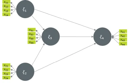
Figure 1 illustrates graphically a simple path model with both reflective and formative models. In this model, the 𝜉3 and 𝜉4 constructs are endogenous variables of the structural model and 𝜉1 and

are its 𝜉2 exogenous constructs. All constructs are estimated based on reflective models except for

𝜉4.

Figure 1 – Example of a simple path model

The graphical connections in the structural model define linear relationships between the constructs, which can be translated in the following equations

𝜉3= 𝛽11𝜉1+ 𝛽21𝜉2

𝜉4= 𝛽12𝜉1+ 𝛽22𝜉2+ 𝛽32𝜉3

More generally, the equations of the structural model are given by: 𝜉𝑖 = 𝛽𝑖0+ ∑ 𝛽𝑖𝑘𝜉𝑘+ 𝜈𝑖

5 Also, the measurement models may be formative or reflective, where formative models are linear regression relationships being the construct the dependent variable, and reflective models are models where it is assumed that the construct impacts the results of the indicator variables. In the reflective measurement model, each indicator variable is related to the constructs by means of a simple regression:

𝑥𝑖𝑗= 𝜛𝑖𝑗0+𝜛𝑖𝑗𝜉𝑖+ 𝜀𝑖𝑗,

where 𝜉𝑖 has mean m and standard deviation 1, where the only hypothesis is that 𝜀𝑖𝑗 has zero

mean and is uncorrelated with its respective construct (Tenenhaus, Vinzi, Chatelin, & Lauro, 2005), such that:

𝐸(𝑥𝑖𝑗|𝜉𝑖) = 𝜛𝑖𝑗0+𝜛𝑖𝑗𝜉𝑖

In the formative measurement model, the construct is generated by its indicators by means of a linear function:

𝜉𝑖 = ∑ 𝜋𝑖𝑗𝑥𝑖𝑗 𝑗

+ 𝛿𝑖

Where the residual vector 𝛿𝑖has a zero mean and is uncorrelated with the indicators. Hence,

𝐸(𝜉𝑖|𝑥𝑖1, … , 𝑥𝑖𝑝_𝑖) = ∑ 𝜋𝑖𝑗𝑥𝑖𝑗 𝑗

+ 𝛿𝑖

Tennenhaus et al. (2005) provide a detailed description of the PLS-PM methodology, including estimation techniques and statistical properties. Henseler, Ringle and Sinkovics (2009) draw from this description and sum it up has follows:

• Step 1: Outer approximation of the latent variable scores. Outer proxies of the latent

variables, 𝜉̂𝑛𝑜𝑢𝑡𝑒𝑟, are calculated as linear combinations of their respective indicators.

These outer proxies are standardized; i.e. they have a mean of 0 and a standard deviation of 1. The weights of the linear combinations result from step 4 of the previous iteration. When the algorithm is initialized, and no weights are available yet, any arbitrary nontrivial linear combination of indicators can serve as an outer proxy of a latent variable;

• Step 2: Estimation of the inner weights. Inner weights are calculated for each latent

variable in order to reflect how strongly the other latent variables are connected to it. There are three schemes available for determining the inner weights;

• Step 3: Inner approximation of the latent variable scores. Inner proxies of the latent

variables, 𝜉̂𝑛𝑖𝑛𝑛𝑒𝑟, are calculated as linear combinations of the outer proxies of their

respective adjacent latent variables, using the aforedetermined inner weights. Step 4: Estimation of the outer weights. The outer weights are calculated either as the covariances between the inner proxy of each latent variable and its indicators (in Mode A, reflective), or as the regression weights resulting from the ordinary least squares regression of the inner proxy of each latent variable on its indicators (in Mode B, formative).

• These four steps are repeated until the change in outer weights between two iterations

drops below a predefined limit. The algorithm terminates after step 1, delivering latent variable scores for all latent variables. Loadings and inner regression coefficients are then

6

calculated in a straightforward way, given the constructed indices and using the formative

and reflective model equations. In order to determine the path coefficients, for each endogenous latent variable a (multiple) linear regression is conducted.

Aside from the linearity constraints addressed by the works of Henseler et al. (2010), Henseler et al. (2012) or Mendes et al. (2018), other problematic concerns have been raised regarding by the original PLS algorithm over time, namely:

• Inconsistency, translated in overestimation of the absolute value of loadings and underestimation of multiple and bivariate(absolute) correlations between the latent variables;

• Lack of an overall goodness of fit measure; • Limitations addressing multicollinearity; • Limitations addressing endogeneity;

However, recent developments in research have addressed these concerns, consolidating the validity of PLS-PM approach.

Dijkstra and Henseler (2015a) presented an improved estimation technique (Consistent PLS – PLSc) that addresses the shortcomings of the original PLS-PM model and leads to consistent and asymptotically normal estimators for the loadings and for the correlations between the latent variables, , by correcting for attenuation of the construct scores correlations with a new and consistent reliability coefficient for PLS. This model has had widespread usage and has become a reference in the estimation of models with reflective indicators (Henseler, Hubona, & Ray, 2016). Also, Dijkstra and Henseler (2015b) have shown that the overall model can be assessed in two non-exclusive ways, by assessing the differences between the empirical and model implied indicator variance-covariance matrix.

Regarding multicollinearity, Jung and Park (2018) proposed the regularized PLSc, which incorporates a ridge type of regularization in the PLSc, an approach that was shown to have interesting results in contexts of strong multicollinearity.

Endogeneity as also been addressed, either by replacing OLS for 2SLS in the structural model (Benitez, Henseler, & Roldán, 2016) or alternative approaches avoiding instrumental variables, which include the Gaussian copula approach (Hult, Hair, Proksch, Sarstedt, Pinkwart, & Ringle, 2018).

Other approaches have been carried to cement the PLS-PM as a solid estimation technique, or a

silver bullet as Hair, Ringle and Sarsted (2011) have classified it.

These works include, namely, a criterion to assess discriminant validity (Henseler, Ringle, & Sarstedt, 2015) designated Heterotrait-Monotrait ratio of correlations (HTMT), new approaches for estimating and testing second-order constructs (see Van Riel, Henseler, Kemeny, & Sasovova, 2017) and multigroup analysis to address groups with different behavior within samples (Chin & Dibbern, 2010; Sarstedt, Henseler, & Ringle, 2011).

7

1.2. PENALIZED SMOOTHING IN THE CONTEXT OF THE PLS

The research developed by Mendes et al. (2018) relaxes the restriction of linearity of the relationships between constructs by allowing the existence of non-linear relationships. By doing so, it proposes an alternative approach by means of penalization.

In this approach the Least Squares objective function is replaced by a penalized version of the traditional objective function. As a way of simplification in the context of one covariate, the objective function will be:

∑𝑛𝑖=1{𝑦_𝑖− 𝑓(𝑥𝑖)}2+ 𝜆 ∫{𝑓′′(𝑢)}2𝑑𝑢 (1)

where

𝑦𝑖 = 𝑓(𝑥𝑖) + 𝜀𝑖

This becomes the traditional setting of a regression with smoothing spline when 𝑓(𝑥𝑖) is

composed a set of pre-defined basis functions such that:

𝑓(𝑥𝑖) = ∑ 𝛽𝑗ℎ𝑗(𝑥) 𝑚

𝑖=1

where the different ℎ𝑗(𝑥) are piecewise polynomials joined together to compose a single smooth

curve. These functions are bounded by points defined as knots of the spline. In the next chapter three alternative sets of basis functions are detailed.

In fact, this setting is based on the framework developed by Reinsch (1967) - which has served as a main reference in fitting non-linear relationships - adapted to a regression context more suited to statistical inference, where the number of functions is not the number of observations, but instead is restricted to a predefined limited number of functions.

The objective function depicted in (1) may be decomposed in two components, where ∑𝑛𝑖=1{𝑦𝑖− 𝑓(𝑥𝑖)}2 minimizes the Euclidean distance, while the second term 𝜆 ∫{𝑓′′(𝑢)}2𝑑𝑢

penalizes overfitting. This second term is 0 if 𝑓 is linear. Also, 𝜆 is a smoothing parameter that controls the trade-off between the two terms, by adding a penalty to the residual sum of squares. Applying this to a SEM context, 𝑦𝑖 is an endogenous latent variable and 𝑥𝑖 may be either an

endogenous or an exogenous variable.

Setting matrix H, where 𝐻𝑖𝑗= ℎ𝑗(𝑥), the spline objective function comes as

(−𝐻𝛽)𝑇_{(−𝐻𝛽) + 𝑛𝜆𝛽}𝑇_Ω𝛽

Where Ω is a matrix of known coefficients comprising the elements of the second derivatives of the basis functions:

8 Mendes et al. (2018) show that differentiating with respect to 𝛽, the estimator of 𝛽 is found through the equation:

𝛽̂ = (𝐻𝑇_{𝐻 + 𝑛𝜆Ω)}−1_𝐻𝑇_𝑦

The added covariance given by 𝑛𝜆Ω depends not only of the shape of the functions, but also the desired amount of smoothing, given by the 𝜆. The largest the 𝜆, less is the weight of the actual data in the fit.

With this configuration, a piecewise continuous linear model is constructed, with the portioning of the range of 𝑥 into K+1 intervals, by choosing K points, called knots, which may be uniformly distributed across 𝑥 or corresponding to specific quantiles.

This means that each individual segment basis functions are summed to obtain a composite function 𝑓(𝑥), which is a cubic spline of order K degrees of freedom.

Wood (2017) provides detailed descriptions of how to estimate models based on natural cubic splines, including the cross-validation methodologies to calculate the optimal 𝜆 (see Wood, 2017, page 255, for a detailed description of cross validation techniques) and strategies to define the number and positioning of the knots. These authors also develop the algorithm in the context of more than one covariate.

The PLSs algorithm

The PLSs algorithm description presented below reproduces (in italic) the PLS algorithm hybrid approach developed by Wold (1982), as presented by Tennenhaus et al. (2005) with the modifications introduced by Henseler et al. (2012) and Mendes et al. (2018):

• Step 1: Calculating outer proxies of latent variable scores: outer proxies of the latent

variables 𝜉̂_𝑗𝑜𝑢𝑡𝑒𝑟are calculated as linear combinations of their respective indicators. The

weights of the linear combinations result from step 4 of the previous iteration or are manually initialized. For each non-linear term, a new proxy is created as the element-wise transformation of the respective outer estimates.

The latent variable scores are estimated as a weighted sum of their respective indicators:

𝑌̂𝑜𝑢𝑡𝑒𝑟 _{= 𝑋𝑊̂}

Where W is the diagonal GxG matrix of the outer weights.

The outer proxies of the latent variable scores are initialised by setting the weights of the previous equation to 1.

Assuming all the MVs, 𝑋1, 𝑋2, ⋯ , 𝑋𝐾 are scaled (𝑚𝑒𝑎𝑛(𝑋𝑖) = 0 𝑎𝑛𝑑 𝑉𝑎𝑟(𝑋𝑖) = 1), the

latent variables are also centered (mean=0) but must be scaled to have unit variance.

Assuming the nonlinear relationship between latent variables are approximated by smoothing splines with K-1 knots (as the constant terms vanish because we are dealing

9 with LVs that have been scaled to mean zero and unit variance) the 𝑛 × 𝐺 matrix 𝑌̂ is

augmented to a 𝑛 × 𝐺(𝐾 − 1) matrix, where the ith _{line is given by:}

𝑌̂_𝑖𝑜𝑢𝑡𝑒𝑟 = [𝑦𝑖1, ℎ(𝑦𝑖1), ℎ(𝑦𝑖1, 𝑦11∗ ), ⋯ , ℎ(𝑦𝑖1, 𝑦1(𝐾−1)∗ ), 𝑦𝑖2, ℎ(𝑦𝑖2), ℎ(𝑦𝑖2, 𝑦21∗ ), ⋯,

ℎ(𝑦𝑖2, 𝑦2(𝐾−1)∗ ), 𝑦𝑖𝐺, ℎ(𝑦𝑖𝐺), ℎ(𝑦𝑖𝐺, 𝑦1𝐺∗ ), ⋯ , ℎ(𝑦𝑖𝐺, 𝑦𝐺(𝐾−1)∗ )]

where the first and second indexes of 𝑦∙∙ refer to the observation and to the LV, and the

first and second indexes of 𝑦∙∙∗refer to the LV variable and the fixed knot (for simplicity we

dropped the superscript “outer"). Moreover, the columns of matrix 𝑌̂should be scaled to

mean zero and unit variance.

• Step 2: Estimation of the inner weights: Inner weights are calculated for each latent

variable in order to reflect how strongly the other latent variables are connected to it. There are three schemes available for determining the inner weights. Wold (1982) originally proposed the centroid scheme. Later, Lohmöller (1989) developed the factor weighting and path weighting schemes. The centroid scheme uses the sign of the correlations between a latent variable or, more precisely, the outer proxy and its adjacent latent variables; the factor weighting scheme uses the correlations. The path weighting scheme pays tribute to the arrow orientations in the path model. The weights of those latent variables that explain the focal latent variable are set to the regression coefficients stemming from a regression of the focal latent variable (regressant) on its latent regressor variables. The weights of those latent variables, which are explained by the focal latent variable, are determined in a similar manner as in the factor weighting scheme. Regardless of the weighting scheme, a weight of zero is assigned to all nonadjacent latent variables.

The inner weights are also determined for each nonlinear term of the splines with K -1 knots.

An illustration of characterization the elements of the augmented matrix of the inner weights 𝐸𝐴𝑢𝑔_{, by means of the centroid method, may be found in Mendes et al. (2018).}

• Step 3: Inner approximation of the latent variable scores: Inner proxies of the latent

variables, 𝜉̂_𝑗𝑖𝑛𝑛𝑒𝑟 , are calculated as linear combinations of the outer proxies of their respective adjacent latent variables, using the afore-determined inner weights. Each term of the splines with K -1 knots is used to estimate the inner proxies of the latent variables.

𝑌̂𝑖𝑛𝑛𝑒𝑟 = 𝑌̂𝑖𝑛𝑛𝑒𝑟𝐸𝐴𝑢𝑔

𝑦̂𝑗𝑖𝑛𝑛𝑒𝑟=

𝑦̂𝑗𝑖𝑛𝑛𝑒𝑟

√𝑉𝑎𝑟(𝑦̂_𝑗𝑖𝑛𝑛𝑒𝑟)

, 𝑗 = 1, ⋯ , 𝐺,

Where 𝐸𝐴𝑢𝑔is the augmented matrix as determined in Step 2.

• Step 4: Estimation of the outer weights: The outer weights are calculated either as the

covariances between the inner proxy of each latent variable and its indicators (in Mode A), or as the regression weights resulting from the ordinary least squares regression of the inner proxy of each latent variable on its indicators (in Mode B).

10 No additional procedure is required in this step because the non-linear terms do not have any assigned indicators, as determined by the hybrid approach.

Mode A: Multivariate regression coefficient with the block of manifest variables as response and the latent variable as the regressor:

𝑤̂𝑗𝑇 = (𝑦̂𝑗𝑖𝑛𝑛𝑒𝑟𝑇𝑦̂𝑗𝑖𝑛𝑛𝑒𝑟) −1

𝑦̂_𝑗𝑖𝑛𝑛𝑒𝑟𝑇𝑋𝑗

= 𝐶𝑜𝑟(𝑦̂_𝑗𝑖𝑛𝑛𝑒𝑟, 𝑋𝑗

Mode B: Multiple regression coefficient with the latent variable as response and its block of manifest variables as regressors:

𝑤̂𝑗𝑇 = (𝑋𝑗𝑇𝑋𝑗) −1 𝑋𝑗𝑇𝑦̂𝑗𝑖𝑛𝑛𝑒𝑟 = 𝑉𝑎𝑟(𝑋𝑗) −1 𝐶𝑜𝑟(𝑋𝑗, 𝑦̂𝑗𝑖𝑛𝑛𝑒𝑟)

These steps are iterated until the change in outer weights between two consecutive iterations falls below a predefined tolerance,

𝑚𝑎𝑥 (|𝑤̂𝑘𝑗

𝑖 _{− 𝑤̂}

𝑘𝑗 (𝑖+1)

𝑤̂_𝑘𝑗(𝑖+1) |) < 𝑡𝑜𝑙𝑒𝑟𝑎𝑛𝑐𝑒, 𝐾 = 1, ⋯ , 𝐾, 𝑗 = 1, ⋯ , 𝐺

The algorithm terminates after step 1, delivering latent variable scores for all latent variables. The loadings and inner regression coefficients are then calculated in a straightforward way, given the constructed indices. The structural relationships are obtained by estimating the additive model using a smoothing spline. For each latent

variable 𝑦𝑗, 𝑗 = 1, ⋯ , 𝐺,we have the following model:

𝑦𝑖𝑗= ∑ 𝛽1 (𝑙)_(𝑦 𝑖𝑙) + #𝑝𝑟𝑒𝑑 𝑙=1 ∑ 𝛽_𝑚+1(𝑙) ℎ𝑚+1(𝑦𝑖𝑙) + 𝜖𝑖𝑗 𝐾−1 𝑚=1

Where 𝑦𝑖𝑗 is an endogenous latent variable, the summation ∑#𝑝𝑟𝑒𝑑𝑙=1 means we are

regressing LV 𝑗 on the set of all predecessor LVs, h is a natural cupic spline and 𝜖𝑖𝑗 are i.i.d.

𝑁(0, 𝜎𝜖2) random variables. The estimated factor scores (including the nonlinear terms) of

the predecessor set of latent variables of 𝑦𝑗are used for this purpose.

In practice the model may be estimated using partial least squares with the mgcv library available through the R Project software (R Core Team, 2018).

Mendes et al. (2018) compare the performance of the PLSs with the PLS and PLSc models and shows that this model performs uniformly better, using absolute bias and Root Mean Squared Error (RMSE) measurements, in a simulated model where structural relationships have underlying real nonlinear functional forms, as proposed by Bauer et al. (2012).

11

1.3. JUSTIFICATION FOR PLS

S

Henseler (2018) reflects on the applications PLS-PM, arguing that this estimation technique is suitable for all main lines of research, namely causal (including confirmatory and explanatory research), exploratory, descriptive and predictive research.

As what regards nonlinearity, Hair et al. (2013) state that nonlinear approaches to PLS-PM must be carried carefully, as results in one specific experiment are not easily replicable and, hence, not generalizable. Also, these approaches are usually more demanding in terms of interpretability. In most contexts, these authors recommend more parsimonious approaches, yielding, in most cases, similar and more easily interpretable results. This is especially the case for causal and experimental research.

As such, the application of PLSs for causal and experimental research is not straightforward and its usage should be taken cautiously. Nevertheless, in these contexts, it shouldn’t, at all, be discarded as an important auxiliary tool, for characterization and visual analysis of results. On the other hand, PLSs appears as a powerful tool for predictive analysis and could become one of the go to tools in specific contexts, such as strategic management, where the main objective is to accurately predict the behavior of out of sample elements and target segment specific policies. In fact, the good performance of this method when compared with PLS and PLSc, as shown be Mendes et al. (2018), regarding absolute bias and RMSE metrics, gives indications that PLSs may be the most suitable to more accurately predict individual behaviors. Also, it shares these models’ properties of transparency in how the prediction is produced, which is a plus when compared with alternative prediction tools (Henseler, 2018).

As Mendes et al. (2018) show in a practical example, visual inspection of the results of PLSs modelling is an important instrument to detect nonlinearity.

Also, the analysis of first, and even second derivatives of the results, provide valuable information about the elements of the population where specific policies may be more impactful in the presence of nonlinearity, allowing for their efficient targeting.

To briefly illustrate this potential, we draw from the application presented by Mendes et at. (2018).

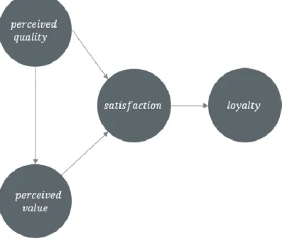
These authors use a real data set produced in the context of the European Customer Satisfaction Index to investigate nonlinear relationships between satisfaction and loyalty and between perceived quality and satisfaction latent variables.

12 The structural equation model is the reduced ECSI model presented below.

Figure 2 – Structural Equation Model of the reduced ECSI

In the table below we also reproduce the indicators of the measurement model of the analysis. All the included indicators are measured on a 10-point scale, from 1 to 10, where 1 traduces a very negative opinion and 10 a very good opinion. Cronbach's alpha (α) and Dillon-Goldstein's rho (ρ) unidimensionality measures are presented for each group of indicators.

Latent variables Manifest variables

Perceived quality

α = 0.93; ρ = 0.94

(a) Overall perceived quality (b) Quality of products and services (c) Customer service and personal advice (d) Availability of contact channels (e) Reliability of products and services (f) Diversity of products and services

(g) Clarity and transparency of information provided (h) Accessibility

(i) Quality of physical facilities

Perceived value

α = 0.91; ρ = 0.95 (a) Evaluation of prices given quality (b) Evaluation of quality given prices

Customer satisfaction

α = 0.84; ρ = 0.91

(a) Overall satisfaction (b) Fulfillment of expectations (c) Distance to ideal company

Customer loyalty

α = 0.89; ρ = 0.95 (a) Intention to remain customer (b) Recommendation to friends and colleagues

Table 1 – Measurement model of the reduced ECSI.

The authors show that the PLSs method behaves slightly better than the PLSc and significantly better than the traditional PLS approach, in that regards R-squared values.

The study presents the estimated relationships of the latent variables graphically. In particular, the visual inspection of the data and estimation results shows the ability of the PLSs to capture

13 apparent non-negligible nonlinearities in the case of the direct relationship between satisfaction and loyalty. Figure 3 illustrates these conclusions, whereby the PLSs fitting is represented by the continuous line.

The results presented by Mendes et al. (2018) are interesting and show the potential of the model for further graphical analysis.

Figure 3 – Estimated direct relationships between Satisfaction and Loyalty in the reduced ECSI model. Circles (∘) represent the traditional PLS estimated factor scores. Crosses (x) represent Smooth PLS estimated factor scores. The (non)-linear relationship estimated using Smooth PLS is represented by the red solid line. PLS and PLSc linear relationships are represented by the blue dashed line and green long-dashed lines.

Going somewhat further, below we present a depiction of the derivatives of the estimated direct relationships between satisfaction and loyalty, alongside the estimated curves produced by Mendes et al. (2018).

The concave form of the direct relationship is evidently translated in a downward line of the derivatives. In fact, this illustrates that targeted satisfaction-based policies applied toward loyalty increase are likely to have a much stronger impact in elements of the population where satisfaction is lower than in those clients that already show high levels of satisfaction.

14 Figure 4 – Estimated direct relationships between Satisfaction and Loyalty and their derivatives

in the reduced ECSI model

In instances where nonlinear direct relationships between variables show inflections in the rate of variation (from concave to convex or vice-versa), inspection of second derivatives should also prove useful to detect the respective inflection points.

Surely, consumer behavior analysis for targeted policies definition shouldn’t forego other sources of information regarding satisfaction and loyalty (e.g. regarding client value), but in marketing research and strategic management perspectives the PLSs produces valuable auxiliary and complementary insights towards efficiently addressing and predicting consumer behavior.

15

1.4. ALTERNATIVE SMOOTHING SPLINES

As stated by Wood (2017), penalised regression splines are low rank smoothing splines, that are designed to provide efficient compromise between retaining the good properties of splines and computational efficiency.

In this section, we present a brief description of the three alternative smoothing methods based on penalized regression splines used in our analysis.

Natural cubic splines

First, we start by presenting the natural cubic regression splines used by Mendes et al. (2018) in their PLSs study, which is drawn from Wahba (1990).

The basis functions in this case are: ℎ1(𝑥) = 1 ℎ2(𝑥) = 𝑥 ℎ𝑖+2(𝑥, 𝑥1) = (𝑥 − 𝑥𝑖)+3 − (𝑥 − 𝑥𝑖)+3 𝑥𝑛− 𝑥𝑖 −(𝑥 − 𝑥𝑖)+ 3 _{− (𝑥 − 𝑥} 𝑖)+3 𝑥𝑛− 𝑥𝑛−1

Where (∙)+ is the positive portion of its argument:

(𝑥 − 𝑥_𝑖)₊= {𝑥 − 𝑥_0, 𝑖, 𝑥 − 𝑥_{𝑥 − 𝑥}𝑖 ≥ 0

𝑖 < 0

In a comparison analysis with other penalized regression splines, Wood (2006) states that the main advantages of natural cubic splines are the fact these are computationally cheap and have directly interpretable parameters. Its main disadvantage is the dependence on knots, which adds a degree of subjectivity in the model design.

P-Splines

P-Splines were introduced by Eillers, & Marx (1996) and are a low rank version of the B-Splines developed by Boor (2001).

Eillers et al (1996) propose the following objective function with basis splines of any order q:

∑ {𝑦𝑖− ∑ 𝑎𝑗𝐵𝑗(𝑥𝑖) 𝑚 𝑗=1 } 2 + 𝜆 ∫ ∑ (∆𝑘𝑎𝑗)2 𝑚 𝑗=𝑘+1 𝑛 𝑖=1

Where the B-splines basis functions of order q are defined recursively: 𝐵_𝑗𝑞(𝑥) = 𝑥 − 𝑥𝑗 𝑥𝑗+𝑚−+1− 𝑥𝑗 𝐵_𝑗𝑚−1(𝑥) + 𝑥𝑗+𝑚+2− 𝑥 𝑥𝑗+𝑚+2− 𝑥𝑗+1 𝐵_𝑗+1𝑚−1(𝑥) 𝑗 = 1, . . . 𝑚 And 𝐵𝑗−1(𝑥) = {1 𝑥₀ 𝑖_{𝑜𝑡ℎ𝑒𝑟𝑤𝑖𝑠𝑒}≤ 𝑥 ≤ 𝑥𝑖+1

16 That is, the authors propose to base the penalty on higher order finite differences of the coefficients of adjacent B-splines. By doing this, the dimensionality of the problem is reduced from the number of observations to the number of B-splines.

The authors describe P-splines as also not being computationally expensive, including for cross-validation (indispensable for calculating 𝜆). These splines have no boundary effects, conserve moments (means, variances) of the data, and have polynomial curve fits as limits. The main limitations of P-splines are the fact that they require equally spaced knots and the interpretation of penalties is far from being straightforward (Wood, 2006).

Thin-plate regression splines

The third type of penalized splines tested in this analysis is Thin Plate Regression Splines (TPRS). TPRS were first introduced by Wood (2002) and built from the Thin Plate Splines (Duchon, 1977). The following paragraphs follow very closely the description and notation carried by Wood (2016)

In thin plate splines smoothing, the objective function to be minimized is: ‖𝑦 − 𝑓‖2_{+ 𝜆𝐽}

𝑚𝑑(𝑓) (2)

Where 𝑓 is a function of the covariates and 𝐽 is a penalty functional measuring the wiggliness of 𝑓 and 𝜆 𝑖𝑠 𝑎 𝑠𝑚𝑜𝑜𝑡ℎ𝑖𝑛𝑔 𝑝𝑎𝑟𝑎𝑚𝑒𝑡𝑒𝑟. 𝑇ℎ𝑒 𝑤𝑖𝑔𝑔𝑙𝑖𝑛𝑒𝑠𝑠 penalty may be written as:

𝐽𝑚𝑑 = ∫. . . ∫ ∑ 𝑚! 𝜈1!. . . 𝜈𝑑! ( 𝜕 𝑚_𝑓 𝜕𝑥₁𝜈1_{. . . 𝜕𝑥} 𝑑 𝜈𝑑) 2 𝑑𝑥1. . . 𝑑𝑥𝑑 𝜈1+...+𝜈𝑑=𝑚 ℝ𝑑

where d is the number of covariates.

Defining m such that 2𝑚 > 𝑑 + 1, function (2) may be written as:

𝑓̂(𝑥) = ∑ 𝛿𝑖𝜂𝑚𝑑(‖𝑥 − 𝑥𝑖‖) + ∑ 𝛼𝑗𝜙𝑗(𝑥) 𝑚

𝑗=1 𝑛

𝑖=1

where 𝛿 and 𝛼 are vectors of the coefficients to be estimated, with 𝛿 being subject to the constrains 𝑇𝑇𝛿 = 0, where 𝑇𝑖𝑗 = 𝜙𝑗(𝑥𝑖) and 𝜂𝑚𝑑(𝑟) = { (−1)𝑚+1+𝑑 2⁄ 22𝑚−1_𝜋𝑑 2⁄ _{(𝑚 − 1)! (𝑚 − 𝑑 2⁄ )!}𝑟2𝑚−𝑑𝑙𝑜𝑔 𝑟 𝑑 𝑒𝑣𝑒𝑛 𝛤(𝑑 2⁄ − 𝑚) 22𝑚_𝜋𝑑/2_{(𝑚 − 1)!}𝑟2𝑚−𝑑 𝑑 𝑜𝑑𝑑

At last, by defining the matrix E by 𝐸𝑖𝑗 ≡ 𝜂𝑚𝑑(‖𝑥𝑖− 𝑥𝑗‖), the objective function may be written

as:

17 As Wood (2016) states and describes, thin plate regression splines are based on the idea of truncating the space of wiggly components of the thin plate spline (the components with parameters 𝛿), while leaving the components of zero wiggliness unchanged (the 𝛼 𝑐𝑜𝑚𝑝𝑜𝑛𝑒𝑛𝑡𝑠). The author also defends that the advantages of this approach are the absence of knots and some optimality properties, which regularly translate in better performances than the other spline methods described above. Regarding disadvantages, computational costs in large data sets is the one that may have more impact in the context of our analysis.

18

2. APPLICATION

2.1. DATA DESCRIPTION AND PROCEDURE

To study the best smoothing choices, Monte-Carlo simulations are carried with different smoothers and knot choice placement strategies.

The software implementation and simulation plan, including the population design, will follow the methodology carried by Mendes et al. (2018) in what regards simulated population dimension, methodologies adopted for observation generation and analyzed random sample sizes.

Hence, the underlying conceptual model will follow the functional forms used by Bauer et al. (2012), to incorporate a wide span of nonlinear relationships, with an added true linear relationship to assess to what extent the PLSs method can capture linear relationships.

In the next paragraphs we describe the steps carried to generate the simulation data, following the method implemented by Mendes et al. (2018).

The Monte Carlo procedure follows three steps: 1. Define an underlying true model.

2. Generate random data emerging from the defined model.

3. Use PLSs to estimate the models with different smoothing splines and compare the different approaches using the absolute bias and RMSE.

The defined model consists of one exogenous latent variable and four endogenous latent variables, all depicting different nonlinear relationships with the exogenous latent variable. The chosen functional forms were those used by Bauer et al. (2012). A true linear relationship is added to assess to what extent the PLSs method can capture linear relationships. Figure 5 presents all the designed relationships.

19 Figure 5 – Structural Equation Model implemented in the Monte Carlo simulation

where 𝐼𝜉<0< 0 is the indicator function, taking the value 1 if 𝜉 < 0 and 0 otherwise, and the

disturbances are sampled as follows:

𝜖𝑗∼ 𝑁(0; 0,5); 𝑗 = 1; 2; 3; 4; 5

To ensure consistency in the PLS-PM, the measurement model has a fixed number of five indicators and latent variables with unit loadings:

𝑥_𝑙𝜉 = 𝜉 + 𝛿0, 𝑙 = 1; 2; 3; 4; 5

𝑦 _𝑙𝜂𝑘 _{= 𝜂}

𝑘 + 𝛿𝑘; 𝑘 = 1; 2; 3; 4; 5; 𝑙 = 1; 2; 3; 4; 5

where residual variance 𝛿(.), follows a normal distribution 𝑁(𝜎𝛿2) with 3 different levels of

variance (3, 1 and 0,33), corresponding to communalities of 0.25, 0.50 and 0.75, respectively. The experiment is implemented with different samples sizes, ranging from 50 to 900 observations (namely, 50, 100, 150, 250, 300, 500, 600, 750 and 900).

Following this methodology, three populations of 10 000 units, will be generated (corresponding to the three levels of residual variance).

Then, K = 1000 random samples of size n = 50; 100; 150; 250; 300; 500; 600; 750; 900, are randomly drawn from the three levels of communality.

20

2.2. RESULTS

This section presents the results drawn from our simulation plan.

After generating the samples, SEM models where estimated through PLSs with the three different types of splines using the “gam” function of the mgcv R Package (Wood, 2018).

To analyze the performance of the models, we measured the absolute bias (B) and the RMSE. The calculations of these indicators are given by:

𝐵𝑙 ≈ 1 300∑|𝑔̅𝑖(𝜉) − 𝑔𝑖(𝜉)| 300 𝑖=1 𝑅𝑀𝑆𝐸𝑙≈ 1 𝐾∑ ( 1 300∑(𝑔̂𝑘𝑖(𝜉) − 𝑔𝑖(𝜉)) 2 300 𝑖=1 ) 𝐾 𝐾=1

Where the index l=1,2,3 represents the different sample sizes, and 𝑔̅𝑘(𝜉) = 1

1000∑ 𝑔̂𝑘𝑖(𝜉)

1000

𝑘=1 is

the mean estimated functional relationship between 𝜉and 𝜂(. ) evaluated at a fixed, even grid of 𝑖 = 1, . . . , 300 points in the range of 𝜉, and 𝑔(𝜉) is the known functional relationship (see Mendes et al, 2018).

Regarding the parametrization of the splines, the following configurations were implemented: 1. Natural cubic splines with 10 equidistant knots (GAM function with bs=”cr” and k=10); 2. P-Splines with a 2nd _{order spline basis and a third order difference penalty (GAM function}

with bs=”ps” and m=2).

3. P-Splines with a 3rd _{order spline basis and a third order difference penalty (GAM function} with bs=”ps” and m=3).

4. P-Splines with a 4rd _{order spline basis and a fourth order difference penalty (GAM function} with bs=”ps” and m=4).

5. Thin Plate Regression splines with 2nd _{order derivatives (GAM function with bs=”tp” and} m=2).

6. Thin Plate Regression splines with 3rd _{order derivatives (GAM function with bs=”tp” and} m=3).

7. Thin Plate Regression splines with 4th _{order derivatives (GAM function with bs=”tp” and} m=4).

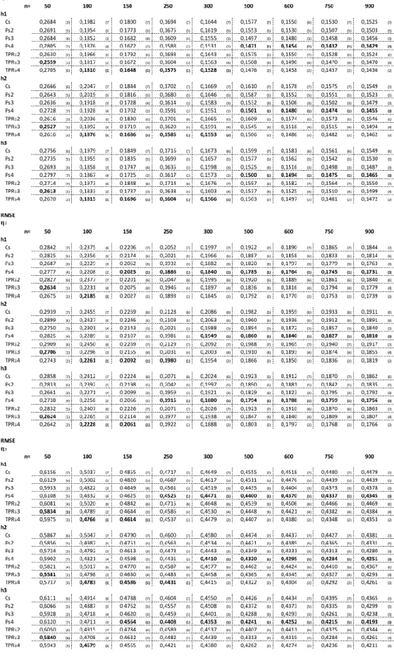
The natural cubic splines configuration is the configuration used by Mendes et al. (2018). Firstly, we compare the performance of splines with 2nd _{order derivatives. Figures 3 and 4 below} compare the performances of these spline configurations across all sample sizes, regarding, respectively, the RMSE and absolute bias.

21 Table 2 - RMSE for Natural Cubic Splines and P-Splines and TPRS with 2nd _{order derivatives}

22 Table 3 - RMSE for Natural Cubic Splines and P-Splines and TPRS with 2nd _{order derivatives} In the context of very small samples (n=50), the results vary depending on the performance indicator. As PLSs with TPRS have less RMSE, the absolute bias (Bias) indicator shows better performances of Cubic Splines and P-Splines depending on the type of nonlinear relationship. However, from n=100 all models with P-Splines perform better in both Bias and RMSE when estimating the relationships 𝜂1 to 𝜂4.

In the specific case of 𝜂5, TPRS have lower RMSE in samples n=100 and 150 and Natural Cubic

Splines show the best Bias results with n=100. Hence, P-Splines tend to be a less obvious choice when the underlying relationship between the latent variables is linear.

23 The results presented in the Annex confirm and deepen these conclusions when splines of higher order are used. In fact, P-Splines fare better in all contexts when the underlying relationships are nonlinear.

This advantage disappears when dealing with a linear relationship. In this case, higher order TPRS present better results than the other cases in what regards RMSE. Regarding Bias performance, the outcome is more mixed and inconclusive. Nevertheless, both TPRS and P-Splines tend to perform better than that natural cubic splines originally employed by Mendes et al. (2018). Hence, with these results, P-splines become the obvious choice for estimating PLSs, since they fare better than the other methodologies in most contexts.

This conclusion is further justified as P-Splines are also faster producing results, as stated by Wood (2016).

Hence, the recommendation drawn from this analysis is that P-Splines should be preferred when using PLSs when nonlinear relationships are present.

24

3. CONCLUSIONS

In the last decade and a half, extensive research in PLS-PM has endowed this estimation technique with an extensive set of tools to overcome or at least mitigate its original shortcomings.

Evenso, nonlinear approaches to PLS-PM have been limited and mostly circumscribed to nonlinear relationships of known functional form.

Building from the work carried by Mendes et al. (2018), which introduces a method that embeds natural cubic splines with fixed knots in the PLS algorithm, aptly named smooth PLS (PLSs), we studied the performance of PLSs with different penalized regression splines.

For that, we embedded the PLS algorithm with P-Splines and Thin Plate Regression Splines in structural model direct relationships, testing different sets of parameters.

The different configurations were tested using a simulated dataset. The simulation framework included four different nonlinear structural relationships and a linear relationship for control purposes. The studied scenarios included six different sample sizes (from n=50 to n= 900), and 3 different levels of communality between latent variables and their indicators.

For comparison of the performance of these configurations we used the usual metrics: Root Mean Squared Error (RMSE) and absolute bias (Bias).

Our results show that P-Splines and TPRS are valid alternatives to natural cubic splines when studying non-linear relationships of unknown form in the context of PLS-SEM. More so, P-Splines fare better than the rest of the configurations in almost all the studied scenarios, except for very small samples contexts (n=50) and linear relationships, where TPRS, in some cases, presented better results.

We also illustrate how PLSs can be a powerful for inspection of nonlinear relationships and be a powerful predictive in corporate management and marketing research work frameworks, namely by assessing first and second derivatives of the direct relationships.

25

4. LIMITATIONS AND FUTURE WORK

Despite the observed trend of better results from P-Splines and TPRS, further simulation work should be developed to test in a more robust fashion whether these splines are significantly better suited to fit nonlinear relationships.

Besides RMSE and Bias, these different parametrizations could also be analyzed in an efficiency perspective. That is, it should be studied whether residual gains in RMSE and Bias with higher order parameters are sufficiently important to compensate in higher estimation times, since the identified differences are residual.

More generally, the full impact of PLSs in predictive research could be object of a structured and detailed approach, namely in what regards the analysis of derivatives of the direct relationships’ functions in the structural model.

Also, the performance of the method in models with formative constructs should be studied to evaluate if the conclusions presented here may be generalized.

As the model behavior hasn’t fared consistently better than the classic PLS approach in contexts where relationships between latent variables are in fact linear, the development of tools to automatically opt for the most adequate model configuration would be a valuable development for practical contexts, since it could provide substantial gains regarding parameter interpretability.

Finally, as the classic PLS has evolved to PLSc to address its original consistency issues, future work on PLSs could pursue a similar path, since the nonlinear approximations carried in this methodology approximation relies on linear combinations of functions.

26

5. BIBLIOGRAPHY

Bauer, D. J., Baldasaro, R. E. & Gottfredson, N. C. (2012). Diagnostic procedures for detecting nonlinear relationships between latent variables Structural Equation Modeling. A

Multidisciplinary Journal, 19(2), 157-177.

Benitez, J., Henseler, J., Roldan, J. (2016). How to address endogeneity in partial least squares path modeling, Proceedings of the 22th Americas Conference on information Systems, 1– 10.

Benitez, J., Henseler, J., Castillo, A., & Schuberth, F. (2020). How to perform and report an

impactful analysis using partial least squares: Guidelines for confirmatory and explanatory IS research. Information & Management, 57(2), 103168.

Boor, C. (2001). A Practical Guide to Splines 2nd _{edition. New York: Springer.}

Chin, W. W., Marcolin, B. L., & Newsted, P. R. (2003). A partial least squares latent variable modeling approach for measuring interaction effects. Results from a Monte Carlo simulation study and an electronic-mail emotion/adoption study. Information Systems

Research, 14, 189 217.

Cortina, J. M. (1993). Interaction, Nonlinearity, and Multicollinearity: implications for Multiple Regression. Journal of Management, 19(4), 915–922.

Dijkstra, T. K. (2010). Latent variables and indices. Handbook of Partial Least Squares: Concepts,

methods and applications. Berlin Heidelberg: Springer, 23–46.

Dijkstra, T.K., & Schermelleh-Engel, K. (2014). Consistent Partial Least Squares for Nonlinear Structural Equation Models. Psychometrika, Volume 79, Issue 4, 585-604.

Dijkstra, T. K., & Henseler, J. (2015). Consistent and asymptotically normal PLS estimators for linear structural equations. Computational Statistics & Data Analysis, 81, 10–23. Dijkstra, T.K., & Henseler, J. (2015). Consistent partial least squares path modeling. MIS

Quarterly , 39(2), 297-316.

Duchon, J. (1977). Splines minimizing rotation-invariant semi-norms in Sobolev spaces.

Constructive Theory of Functions of Several Variables Lecture Notes in Mathematics, 85–

100.

Eilers, P. H. C., & B. D. Marx (1996). Flexible smoothing with B-splines and penalties, Statistical

Science, 11(2), 89–121.

Green, P.J., & Silverman, B.W. (1994). Nonparametric regression and generalized linear models –

A roughness penalty approach. London: Chapman & Hall

Hair, J.F., Ringle, C.M., & Sarstedt, M. (2011). PLS-SEM: indeed a silver bullet. J. Market. Theory

27 Hair, J. F., Ringle, C. M., & Sarstedt, M. (2013). Partial Least Squares Structural Equation

Modeling: Rigorous Applications, Better Results and Higher Acceptance. Long Range

Planning, 46(1-2), 1–12.

Hair, J. F., Sarstedt, M., Ringle, C. M., & Mena, J. A. (2011). An assessment of the use of partial least squares structural equation modeling in marketing research. Journal of the Academic

Marketing Science, 40(3), 414–433.

Hair, J. F., Hult, G. T., Ringle, C. M., & Sarstedt, M. (2014). A primer on partial least squares

structural equation modeling (PLS-PM).Thousand Oaks, CA: Sage.

Henseler, J. (2018). Partial least squares path modeling: Quo vadis? Quality & Quantity, 52(1), 1– 8.

Henseler, J., & Chin, W. W. (2010). A Comparison of Approaches for the Analysis of Interaction Effects Between Latent Variables Using Partial Least Squares Path Modeling. Structural

Equation Modeling: A Multidisciplinary Journal, 17(1), 82–109.

Henseler, J., & Fassott, G. (2010). Testing moderating effects in PLS path models: An illustration of available procedures. Handbook of Partial Least Squares: Concepts, methods and

applications, 713–735.

Henseler, J., Hubona, G., & Ray, P. A. (2016). Using PLS path modeling in new technology research: updated guidelines, Industrial Management & Data Systems, 116(1), 2-20. Henseler, J., Ringle, C. M., & Sinkovics, R. R. (2009). The use of partial least squares path

modeling in international marketing, Advances in International Marketing - New

Challenges to International Marketing, 277-319.

Hult, G. T. M., J. F. Hair, D. Proksch, M. Sarstedt, A. Pinkwart, & C. M. Ringle (2018). Addressing Endogeneity in International Marketing Applications of Partial Least Squares Structural Equation Modeling. Journal of International Marketing, forthcoming.

Jung, S., & Park, J. (2018). Consistent Partial Least Squares Path Modeling via Regularization. Frontiers in Psychology, 9.

Kelava, A., Werner, C. S., Schermelleh-Engel, K., Moosbrugger, H., Zapf, D., Ma, Y., Cham H., Aiken, L. S. & West, S.G. (2011). Advanced nonlinear latent variable modeling: Distribution analytic LMS and QML estimators of interaction and quadratic effects, Structural Equation

Modeling: A Multidisciplinary Journal, 18(3), 465-491.

Klein, A. G. & Moosbrugger, H. (2000). Maximum likelihood estimation of latent interaction effects with the LMS method, Psychometrika, 65(4), 457-474.

Klein, A. G., & Muthén, B. O. (2007). Quasi-maximum likelihood estimation of structural equation models with multiple interaction and quadratic effects, Multivariate Behavioral Research, 42(4), 647-673.

Kline, R. B. (2005). Principles and practice of structural equation modeling, (2nd ed.). New York, NY: Guilford.

28 Lohmöller, J.-B. (1989). Latent variable path modeling with partial least squares. Heidelberg:

Physica.

Marsh, H. W., Wen, Z., & Hau, K (2004). Structural equation models of latent interactions: evaluation of alternative estimation strategies and indicator construction. Psychological

methods, 9(3), 275-300.

Mendes, J., Coelho, P. S., & Hanseler J., (2018). Smooth Partial Least Squares Path Modelling,

forthcoming.

R Core Team (2018). R: A language and environment for statistical computing. R Foundation for Statistical Computing. Vienna: Austria.

Pek, J., Sterba, S. K., Kok, B. E. & Bauer, D. J. (2009). Estimating and visualizing nonlinear relations among latent variables: a semiparametric approach. Multivariate Behavioral

Research, 44(4), 407-436.

Reinartz, W. J., Haenlein, M., & Henseler, J. (2009). An Empirical Comparison of the Efficacy of Covariance-Based and Variance-Based SEM. International Journal of Research in

Marketing , 26(4), 332-344.

Reinsch, C. H. (1967). Smoothing by spline functions. Numerische Mathematik 10, 177–183. Ruppert, D. (2002). Selecting the Number of Knots for Penalized Splines, Journal of

Computational and Graphical Statistics, 11(4), 735-757.

Sarstedt, M., Henseler, J., Ringle, C.M. (2011). Multi-group analysis in Partial Least Squares (PLS) path modeling: alternative methods and empirical results. Advances in International

Marketing 22, 195-218.

Song, X.-Y. & Lu, Z.-H. (2010). Semiparametric latent variable models with Bayesian P-splines, Journal of Computational and Graphical Statistics. 19(3), 590-608.

Song, X.-Y., Lu, Z.-H., Cai, J.-H., & Ip, E. H.-S. (2013). A Bayesian modeling approach for

generalized semiparametric structural equation models, Psychometrika, 78(4), 624-647. Steenkamp, J.-B., & Baumgartner, H., 2000. On the use of structural equation models for

marketing modeling, International Journal of Research in Marketing 17(2-3), 195-202. Tenenhaus, M., Vinzi, V. E., Chatelin, Y-M., & Lauro, C. (2005). PLS path modeling. Computational

Statistics & Data Analysis, 48(1), 159 – 205.

Tuu, H. H., & Olsen, S. O. (2010). Nonlinear effects between satisfaction and loyalty: An empirical study of different conceptual relationships, Journal of Targeting, Measurement and

Analysis for Marketing, 18(3-4), 238–251.

van Riel, A.C., Henseler, J., Kemény, I., Sasovova, Z. (2017). Estimating hierarchical constructs using consistent partial least squares: the case of second-order composites of common factors. Industrial Management & Data Systems 117(3), 459–477.

Wold, H. O. A. (1975). Path models with latent variables: The NIPALS approach. IH. M. Blalock

29 Wold, H. O. A. (1982). Soft modelling: The basic design and some extensions. K. G. Joreskog & H.

O. A. Wold (Eds.), Systems under indirect observation, part II. Amsterdam, The

Netherlands: North-Holland, 1–55.

Wood, S. (2006). Generalized Additive Models: an introduction with R. Boca Raton: Chapman & Hall/CRC Press.

Wood, S. (2017). Generalized Additive Models: an introduction with R. 2nd _{Edition. Boca Raton:} Chapman & Hall/CRC Press.

Wood, S. N. (2018). Package ‘mgcv’ - R.

30

ANNEX – RMSE AND ABSOLUTE BIAS RESULTS

31 Table A.1 (continued) - RMSE for Natural Cubic Splines and P-Splines and TPRS

32 Table A.2 – Absolute Bias for Natural Cubic Splines and P-Splines and TPRS

33 Table A.2 (continued) – Absolute Bias for Natural Cubic Splines and P-Splines and TPRS