NEW TRENDS IN MATHEMATICAL SCIENCES
Vol. 1, No. 1, 2013, p.93-99ISSN 2147-5520 - www.ntmsci.com
The chaotic behaviour on transition points between parabolic
orbits
Cahit Karakuş
1, Ertuğrul Bolcal
1, and Yaşar
Polatoğlu
21Department of Physics Science, Istanbul Kültür University, Bakırköy, 34156, Istanbul TURKEY
2Department of Mathematics and Computer Science, Istanbul Kültür University, Bakırköy, 34156, Istanbul TURKEY
Abstract: The potential energy surfaces interact each other and their curvilinear coordinates have the critical information about disturbance at interaction points. Therefore, transition points between parabolic orbits that are solutions of one differential equation with variable coefficients is studied in this paper. Also we present an approach for the chaotic behaviour on transition points of the parabolic orbits.
Keywords: Chaotic Behaviour, Differential Equation, Parabolic Intersections, Quadratic Function, Schwarzian Derivative,
1. Introduction
A dynamical system determines the present state in terms of past states and is described by equations representing the evolution of a solution with time, initial conditions and control signals [1]. The Intersections of parabolic orbits play an important role in analysis, design and synthesis of control laws in dynamical systems. In an elliptical or circular orbit, the planet is moving slower than the escape velocity. One focus of the ellipse is on or near the primary and the second focus is on an unoccupied point in space. A planet in this type of orbit will continue to orbit the primary unless another force alters its path. All planets and moons in solar system follow this type of orbit. In a parabolic orbit, the planet has reached escape velocity. A planet with this type of orbit will never return to orbit the primary again. Also in a hyperbolic orbit, which is somewhat more flattened than a parabolic orbit, the planet is moving faster than escape
velocity. A satellite leaving earth’s orbit will follow parabolic or hyperbolic path [2-8].
The interactions points on intersection from a parabola orbit to other will be computed in this study. A parabola is quadratic function. If the quadratic equations are the solutions of the same differential equation with variable coefficients, the points of intersection between orbits give knowledge about the interactions and transitions. Furthermore, these equations have two distinct real roots. Hence, the chaotic behaviour of the transition between the points of parabolic intersections will be studied by using the methods of Schwarzian Derivative, Lyapunov Exponent and Bifurcation Diagram [9-16].
2. The parabolas which are the solutions of differential equation with variable coefficients
A quadratic function is 2 ( ) =
f x ax bxc, where x is path-dependent variable and a b, , and c are constants. In this study, we assume that, a> 0, c only changes the vertical position. The quadratic equations which have distinct real roots, open upward and downward structure are given (1) and (2).
2
1( ) = ( )
f x ax a c x c (1)
2
2( ) = ( )
We assume that (1) and (2) are the solutions of second order differential equation with variable coefficients as given below,
''
( ) ( ) ( ) ( ) = 0
f x p x f x q x (3)
We have to verify that if f x1( ) and f x2( ) are the solutions of equation in (3). Further, to determine the coefficients of
( )
p x and q x( ), we substitute f x1( ), f x2( ), ''
1( )
f x and ''
2 ( )
f x into the differential equations in (3), and eventually obtain (4) and (5)
''
1( ) ( ) ( )1 ( ) = 0
f x p x f x q x (4)
and
''
2( ) ( ) 2( ) ( ) = 0
f x p x f x q x (5)
Where ''
1( )
f x and ''
2( )
f x are the second order derivatives of the f x1( ) and f x2( ) respectively. '' 1( ) = 2
f x a, f x1( ), quadratic function opens upward and ''
2( ) = 2
f x a, f x2( ), quadratic function opens downward (a>0). Variable coefficients p x( ) and q x( ) are obtained from (4) and (5),
2 2 ( ) = , p x x x (6) 2 ( ) = c,
q x x
(7)
= 1.
c (8)
If we substitute p x( ), q x( ) and c in to the differential equation with variable coefficients as given (3), the differantial
equation is therefore,
2
2 2
( ) 2 2
( )
d f x
f x x
dx x x (9)
The solutions of the differential equation in (9) are found as (10) and (11).
2
1( ) = ( 1) 1
f x ax a x (10)
2
2( ) = ( 1) 1
f x ax a x (11)
The roots of the parabola equation f x1( ) are 1 1 ,
a
, and the roots of the parabola equation f x2( ) are 1 1 ,
a
, where a>0. As shown in Fig.1, the transition points of parabolas affect each other.
3. Chaotic behaviour on the transition points of parabolas
3.1. Schwarzian derivative
2
''' ''
' '
( ) 3 )
( ) =
2
( ) ( )
f x f x
Sf x
f x f x
(12)
where f x'( ) , f''( )x
, f'''( )x
denote the first, second and third order derivatives of the f x( ) at x, respectively. If
( ) < 0, ( )
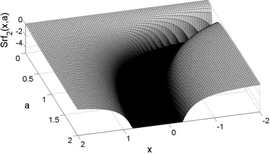
Sf x f x will have a chaotic behaviour on x and a values. Schwarzian Derivatives (13), (14) of functions,
1( )
f x and f x2( ) as given (10) and (11) that are solutions of the differantial equation (9) are calculated bu using (12).
2-dimensional shapes are given in Fig. 2 and Fig. 3.
2 1 2 6 ( ) = (2 1) a Sf x ax a
(13)
2 2 2 6 ( ) = (2 1) a Sf x ax a
(14)
Schwarzian Derivatives Sf x1( ) and Sf x2( ) of f x1( ), and f x2( ) approach to highly chaos, between x0 and x1 in
x-axis while a is getting greater.
3.2. Sensitive dependence on initial conditions
Lyapunov exponents of a dynamical system provide a quantitative measure of its sensitivity to initial conditions. The average rate of convergence or divergence of the system along the axes in phase space gives Lyapunov Spectrum of the map. We focus on the calculation of Lyapunov exponents in the current context of one-dimensional discrete maps. The Lyapunov exponent measures the exponential rate at which neighboring orbits are moving apart. It is determined by averaging the natural logarithm of the derivative evaluated along an orbit. If a dynamical system has sensitive dependence on initial conditions that is a typical x0 is a sensitive point, then it cannot be used to predict for large time,
because there are errors in numerical calculations. Hence this is an important concept for chaos. More precisely, let
( )
f x be a map on R, a point x0 has sensitive dependence on initial conditions, if there is a constant d> 0, such that for any ( ) > 0n , there is an x satisfying |xx0|< ( ) n and an integer k, such that | ( ) ( 0) |
k k
f x f x d. Let fk
denotes the kth iterate of f x( ) . For simplicity, we call such a point x0 a sensitive point. If the initial condition is unstable, small errors or perturbations in the state would cause the orbit to move away from the fixed point.
We focus on the calculation of Lyapunov exponents in the current context of one-dimensional discrete maps [11-15]. Lyapunov exponents measure the rate of divergence of orbits originating from arbitrarily close initial conditions. That
is, they measure a system’s sensitivity to its initial conditions. A positive Lyapunov exponent indicates that the system is chaotic. f x1( ) and f x2( ), which are the solutions of the same non-linear dynamic system by given in (9) with initial
condition x0. Examine a small perturbation of this starting point, defined by x00, where the initial separation 0 is
assumed to be very small. Suppose n is the separation after n iterations of the system. If | | | 0|
n
n e
, then is called a Lyapunov exponent. Lyapunov exponents can be found, for a trajectory starting at x0, from the limit. The
exponents are described as [15],
1
=0 1
=lim[ | ( ) |]
n
i
n i
ln f x n
(15)n is the number of iteration of the dynamical system and x0 is the initial condition. Further details can be found in [15].
It is clear from (15) that ìs depends on the starting point x0. In practice, the value of converges after a few hundreds iterations: 1 =0 1 | ( ) | N i i
ln f x N
< 0
, the system attracts to a fixed point or stable periodic orbit. These systems are non conservative (dissipative) and exhibit asymptotic stability. = 0, the system is neutrally stable. Such systems are conservative and in a steady state mode. They exhibit Lyapunov stability. > 0, the system is chaotic and unstable. The exponents of f x1( ) and f x2( ) are given by (16),
1
1
=0 1
( ) | 2 ( 1) |
N
i i
a ln ax a
N
(17)1
2
=0 1
( ) | 2 ( 1) |
N
i i
a ln ax a
N
(18)Fig. 4 shows the Lyapunov exponent computed for the map with a ranging from 0 to 2. For each value of a, (17) and (18) is estimated using N= 1000, with an initial starting point of x0= 0.5. This spectrum is invariant in a basin of attraction, and so will only vary in different regions of stability. In the current case, the signal is entirely chaotic, and then undergoes periodic transitions from chaos to stability, as a increases. Fig.4 shows the Lyapunov exponent computed for the f x1( ) and f x2( ), for 0 <a< 2. We notice that remains negative for a< 1.6, and approaches 0 at
the period doubling bifurcation.
A bifurcation diagram gives the value and stability of the steady state and periodic orbits. In bifurcation diagram, for each value of a is reported the local maximum of values of xn. The transition from one regime to another is called a
bifurcation [16]. A point in a bifurcation diagram where stability changes from stable to unstable is called a bifurcation point. A bifurcation occurs when a small smooth change made to the parameter values (the bifurcation parameters) of a system causes a sudden qualitative or topological change in its behaviour.A bifurcation is a sudden change in the number or nature of the fixed and periodic points of the system[17]. Fig.5 shows the stability of the solution as a function of a, and then its transition to unstable and chaotic behaviour. One way of summarizing the range of behaviours encountered whenaincreases is to construct a bifurcation diagram. Such a diagram gives the value and stability of the steady state and periodic orbits (Fig.5). In this diagram, for each value of a is reported the local maximum of values of xn. The transition from one regime to another is called a bifurcation. Further system parameter
changes are shown to result in even more extreme changes in behaviour, including higher periodicity, quasiperiodicity and chaos. Let f x1( ) = f x a1( , ) and f x2( ) = f x a2( , ), where a is a scalar parameter. The variable x is on the vertical
axis, and the bifurcation parameter a is on the horizontal axis. As shown in Fig.5, transitions start between parabolas which is given (10) and (11) that are different solutions of one differential equation (9) with variable coefficients, when
x goes to 0.5 and a is greater than 1.6.
4. Conclusion
In this paper, we present a approach for the characterization of the points on parabolic intersection seams as either local minimum or saddle points using same second order differential equation. The curvilinear coordinates are conceptually important, they also give rise to additional practical applications; electromagnetic coupling, vibration, turbulence, absorption, molecular motions. The parabolic intersections are not isolated points but rather are part of an extended seam of geometries where the energy of two states varies while preserving their degeneracy. Finally, the chaotic behaviour of strong interactions of parabolic intersections can be determined by using the methods of Schwarzian Derivative, Lyapunov Exponent, Bifuracation Diagram and these methods show good results.
References
[1]J.M.Jirstrand. Nonlinear Control System Design by Quantiier Elimination, J. Symbolic Computation, 24, 137-152, August, 1997, pp: 137-152.
[2]F.Sicilia, L.Blancafort, M. J. Bearpark, and M. A. Robb. Quadratic Description of Conical Intersections: Characterization of Critical Points on
the Extended Seam. J. Phys. Chem. A111, 2007, pp:2182-2192.
[3]H.Riecke. Methods of Nonlinear Analysis 412 Engineering Sciences and Applied Mathematics. Northwestern University, 2008.
[4]R.M. May. Simple Mathematical Models with very Complicated Dynamics. Nature, 1976, pp:261 459-67.
[5]M.J. Bearpark, M. A. Robb, H. B. Schlege. A direct method for the location of the lowest energy point on a potential surface crossing.
[6]M. J. Paterson, M. J. Bearpark, and M. A. Robba. The curvature of the conical intersection seam: An approximate second-order analysis.
Journal of Chemical Physics. Volume 121, Number 23. 15 December 2004.
[7] D. A. Brue, X. Li, and G. A. Parker Conical intersection between the lowest spin-aligned Li3(4A)… potential-energy surfaces. Journal of
Chemical Physics.123, 091101, 2005.
[8] B. G. Levine, C. Ko, J. Quenneville and T. J. Martinez Conical intersections and double excitations in time-dependent density functional
theory. Molecular Physics, Vol. 104, Nos. 5–7, 1039–1051, 10 March–10 April 2006.
[9]M.W. Hirsch, S.Smale, R.L. Devaney. Differential Equations, Dynamical Systems and Introduction to Chaos., Elsevier Academic Press, 2004.
[10] J. S. Kozlovski. Getting rid of the negative Schwarzian derivative condition, Annals of Mathematics, 152 (2000), 743-762.
[11]J T.R. Scavo, J. B. Thoo. On the Geometry of Halley’s Method, The American Mathematical Montly, 1994.
[12]L.-S. Yao Computed chaos or numerical errors. Nonlinear Analysis: Modelling and Control, Vol. 15, No. 1, 2010, pp: 109-126.
[13]H. Kocak, K. J. Palmer Lyapunov Exponents and Sensitive Dependence. J Dyn Diff Equat, 22, 2010, pp:381-398.
[14]T. Theivasanthi Bifurcations and chaos in simple dynamical systems. International Journal of Physical Sciences Vol. 4 (12), December,
2009, pp. 824-834.
[15]J G. V. Weinberg and A. Alexopoulos. Examples of a Class of Chaotic Radar Signals, ISBN 0-387-94677-2.
[16]J. K.T.Alligood, T.Sauer, J.A.Yorke. CHAOS An Introduction to Dynamical Systems, Elsevier Academic Press, Chapter:11, Page:447-496,
ISBN 0-387-94677-2, 2000.
[17]E. R. Scheinerman. Invitation to Dynamical Systems,Department of Mathematical Sciences The Johns Hopkins University, Chapter:4.2,
Page:127-136, ISBN 0-13-185000-8, 2000.
Figure 1: The Interactions Between Surfaces of Parabolic Intersections, f x f x1( ), 2( ), for various a
Figure 2: Schwarzian Derivative of f x1( ) for various a
Figure 3: Schwarzian Derivative of f x2( ) for various a
Figure 4: The Lyapunov Exponent for 0 <a< 2,f x and f x1( ) 2( ) for x0= 0.5