ABSTRACT: This article deals with the problem of Earth’s magnetic ield sensors calibration in the context of low-cost nanosatellites’ navigation systems. The attitude of space vehicles can be determined from the state estimation using information from three-axis inertial and non-inertial sensors. This study considers a three-axis solid-state magnetometer. In the vehicle itself, the presence of ferrous materials and electronic devices creates disturbances, distorting the measured ield. The sensor precision can be enhanced through calibration methods which calculate the systematic error. The objective here is to study and implement calibration combining a geometric method and the TWOSTEP algorithm. The methodology is based on numerical simulations, with the development of a database of the Earth’s magnetic ield along the vehicle orbit, and experimental tests using a nanosatellite mockup, containing an embedded processor Arduino MEGA 2560 platform and the magnetometer HMC5843.
KEYWORDS: Nanosatellites, Attitude, Navigation systems, Magnetometer calibration, TWOSTEP algorithm.
Experimental Magnetometer Calibration
for Nanosatellites’ Navigation System
Jader de Amorim1, Luiz S. Martins-Filho1
INTRODUCTION
A crucial requisite for an artiicial satellite is the control of its spatial orientation, generally called attitude. he attitude must be stabilized and controlled for various reasons, concerning the spacecrat operational functions, like the correct antenna pointing for the communication, the appropriate orientation related to the Sun for the thermal control, and many others. he tasks associated to the satellite mission also demand the accuracy in the orientation of sensors and other devices for a suitable performance. Several phenomena can cause inaccuracies on the space vehicle orbit and attitude. In order to have the spacecrat controlled, the attitude must be known through the various stages of its life cycle. From the launch to inal service orbit, the space vehicle attitude should be determined (Pisacane 2005).
Attitude determination implies the measurement of any quantity sensitive to the attitude. One of the most used phenomena in the determination procedures is the Earth’s magnetic ield. he local geomagnetic ield vector is frequently one of the attitude information sources. A magnetometer measures the strength of a magnetic ield in one, two or three directions. If Bk is the value of a magnetic ield in the spacecrat body coordinate system, as determined from the magnetometer in the time tk, and Tkis the known value of the magnetic ield in the inertial coordinates, then a simple model is (Pisacane 2005):
1.Universidade Federal do ABC – Centro de Engenharia, Modelagem e Ciências Sociais Aplicadas – Santo André/SP – Brazil.
Author for correspondence: Luiz S. Martins-Filho | Universidade Federal do ABC – Centro de Engenharia, Modelagem e Ciências Sociais Aplicadas | Avenida dos
Estados, 5.001 – Bangu | CEP: 09.210-971 – Santo André/SP – Brazil | Email: [email protected]
Received: 12/16/2015 | Accepted: 01/29/2016
where: Ak is the rotation matrix describing the attitude. hus the measurement of the magnetic ield provides a measurement of the attitude relative to inertial coordinates. he vector is generally given by a geomagnetic reference ield (1)
model, which requires knowledge of the spacecrat position. he magnetometer does not measure the magnetic ield in the body frame but in a frame ixed in the magnetometer. he measured magnetic ield in the body frame is obtained from the measured ield in the sensor frame according to:
(Caruso 2000) and TWOSTEP (Alonso and Shuster 2002), respectively for ground and in-light procedures.
THE MAGNETOMETER CALIBRATION
ALGORITHMS
The magnetometer determines the direction and the magnitude of the magnetic field with several operational advantages such as low weight, small power consumption, and no moving parts; therefore, it does not interfere with vehicle dynamics. he main problem of this instrument is the low accuracy of its measurements as a function of considerable errors from Earth’s magnetic ield model.
Besides, the accuracy of the magnetometer can be disrupted by a series of magnetic disturbances generated in the spacecrat. he TWOSTEP algorithm was developed to determine the bias, i.e. the measurement systematic error. Besides, the accuracy of the magnetometer can be disrupted by a series of magnetic disturbances generated in the spacecraft. The TWOSTEP algorithm was developed to determine the bias, i.e. the measurement systematic error. Some algorithms have been proposed to avoid this type of calculation.
GEOMETRICAL CALIBRATION APPROACH
he irst approach for the magnetometer calibration is an extension of the method proposed in Caruso (2000) and is developed as an application note for the LSM303DLH sensor module (ST Microelectronics 2012). Considering a tridimensional space, the relation between the geomagnetic ield (Hx, Hy, Hz) and the measurements vector (Bx, By, Bz) can be expressed as: where: Smag k is the magnetometer alignment matrix, a proper
orthogonal matrix that transforms representations from the magnetometer frame to the body frame.
Moreover, measurement of the magnetic ield alone is not suicient to determine the attitude. herefore the magnetic ield measurement, although a vector, has only two degrees of freedom that are sensitive to the attitude (namely, the direction). Since we need three parameters to specify the attitude, one vector measurement is not enough. Other sensors, e.g. the Sun sensor, are used to complete the necessary information to determine the attitude.
In the literature, there are a number of studies around the subject of magnetometer calibration. For instance, Juang et al.
(2012) deals with the problem of magnetometer data based on orbit determination and the sensor calibration. he proposed solution applies an unscented Kalman ilter for estimation of satellite position and velocity. he results show the adequacy of the extension strategy of orbit determination algorithm to the problem of magnetometer calibration. In Inamori and Nakasuka (2012), in the context of a scientiic nanosatellite mission, the magnetometer calibration algorithm is also based on the unscented Kalman ilter.
hree diferent algorithms are tested in terms of performance and computational costs in Crassidis et al. (2005): the TWOSTEP (Alonso and Shuster 2002), the extended Kalman ilter, and the unscented Kalman ilter. he study presented in Vasconcelos
et al. (2011) formulates a maximum likelihood estimator to an optimal parameter calibration without using external attitude references. he proposed calibration procedure corresponds to an estimation of rotation, scaling and translation transformation and represents an interesting tridimensional reinement of the geometric method proposed in Caruso (2000).
he purpose of our study is to implement and evaluate two procedures in a quite simple and low-cost experimental setup. One dedicated to ground calibration and the other, to in-light calibration. he adopted strategies, based on the precedent studies discussed above, are the geometric method
where: Mm is the misalignment matrix (between magnetic ield and sensor frame axes); xsf, ysfand zsf are the scale factors;
bx, byand bz are the systematic errors due to strong magnetic disturbances (bias); and Msi is a matrix that represents the weak magnetic distortion.
he calibration procedure can be done by data acquisition during rotations around the three axes (X, Y, Z) or randomly combined rotations (ST Microelectronics 2012). In the case of presence of strong or weak magnetic distortions, the measurement
ˆ
ˆ
ˆ
(2)will reproduce these disturbs by a bent and displaced ellipsoid. his calibration procedure is able to compensate these disturbs that are solidary with the satellite body and to allow the magnetometer to measure the external ield. An example of graphical representation of measurements taken during tridimensional and planar rotations is shown in Fig. 1. In this case, the sensor measurement is clearly afected by internal disturbances. he ellipsoid can be described by:
the parameters xsf, ysf, zsf, bx, by and bz. Ater these adjustments, the graphic representation of calibrated magnetometer data becomes a unitary sphere (Fig. 2).
where x0, y0 and z0 are ofsets of bx, by and bz caused by the strong magnetic distortion; x, y and z are the measurements (Bx, By, Bz); a1, a2 and a3 are the lengths of ellipsoid semi axes;
a4, a5 and a6 represent the efects of cruised axes measurements, responsible for the ellipsoid inclination; and R is a geomagnetic ield constant.
Figure 1. The geomagnetic ield measure before sensor calibration (mG) (Alonso and Shuster 2003).
Figure 2. The geomagnetic ield measure after sensor calibration (mG) (Alonso and Shuster 2003).
When the weak magnetic distortion is negligible, the ellipsoid is not bent and Msi is an identity matrix. Consequently, Eq. 4 can be simpliied as follows:
And the least square method provides the adjustment of the magnetometer data to the equation of an ellipsoid by determining
Equation 5 can be rewritten as:
Consequently, the non-calibrated magnetometer data (Bx, By, Bz) can be combined into a matrix N× 6 dimentional, T, where N is the number of measurements (N ≠ 0 and N∈ N). Then, Eq. 6 becomes:
The parameter vector U can be determined using least squares method (ST Microelectronics 2012):
hen, (4)
(5)
(6)
(7)
(8)
(9)
where: U(i), i= 1, ..., 6, are the components of U. Taking the diferences,
process. hrough this mathematical operation, the highest order term of the cost function can be eliminated, inding a simpliied mathematical model (Alonso and Shuster 2002). A more complete mathematical model of the magnetic ield vector measurement is given by (Kim and Bang 2007):
Equation 5 becomes:
Finally, the scale factors for calibration can be computed:
THE TWOSTEP ALGORITHM
A method to estimate the magnetometer systematic error without the knowledge of the ship attitude is the verification scale, which minimizes the differences of the squares of the magnitudes from measured and modeled magnetic fields. The scalar verification is based on the principle that parameters, such as the magnitude of a vector, do not depend on the coordinate system. However, the disadvantage of this approach is that the resulting cost function to be minimized is an equation of the fourth degree with respect to the bias vector. Some algorithms have been proposed to avoid this type of calculation. The TWOSTEP algorithm is an improvement of these methods, by discarding less data during the centering
where: b is the magnetometer measurement systematic error (bias); εk is the measurement noise considered, for simplicity, white and Gaussian, whose covariance matrix is Σk.
Minimization of Measurement Systematic Error
For the scalar veriication, the equations are deined as follows (Kim and Bang 2007):
where: zk is deined as actual measurement and vk is deined as the efective noise measurement.
he negative log-likelihood function of magnetometer bias vector is given by Alonso and Shuster (2003):
where: μvk is the mean and σvk2 is the variance of the efective
measurement noise, considered as Gaussian for simplicity;
zkʹis the real value of zk.
where: tr(Σk) is the trace of matrices function.
The Centering Operation
By means of a mathematical operation called centering, the term of highest order can be removed. herefore, the following weighted averages are deined (Alonso and Shuster 2002): (10)
(13)
(14)
(18)
(19)
(20)
(21)
(22)
(23)
(24) (15)
(16)
(17) (11)
herefore:
2.From the centered estimate, b*, calculate Fbb and Fbb through the above equations and the following equation:
he following centered quantities are deined:
hat implies in (Alonso and Shuster 2002):
The Procedure of the TWOSTEP Algorithm
he TWOSTEP algorithm, as the name implies, consists of two steps. In the first step, the centered magnetometer systematic error estimate is calculated, as well as its covariance matrix. he need of an additional correction step due to the discarded central term is measured by a direct comparison of the centered and central Fisher information matrices. In the step two, the obtained centered bias vector value is used as an initial estimate. he TWOSTEP algorithm can be described by Alonso and Shuster (2003):
Step one
1. Calculate the centered estimate of the magnetometer systematic error, b*, and the covariance matrix, Pbb, using data from the centered quantities and the equations:
where: Fbb and Fbb are the Fisher information matrices. If the diagonal elements of Fbb are suiciently smaller than the diagonal elements of Fbb ([Fbb]mm < C [Fbb]mm, m = 1,2,3), the calculation of the magnetic ield systematic error vector can be terminated at that point, and b* can be accepted as the best estimated value. he covariance matrix of the estimated error will be the inverse of Fbb.
Step two
1. If the inequality from the previous step is not true, use the centered value b* as an initial estimate. he correction due to the central term is computed using the Gauss-Newton method:
he Fisher information matrix (Fbb) is given by the equation:
where the gradient vector g(b) is given by:
2. The previous step is repeated until ηii is less than a predetermined value, where:
In this study, the adopted stopping criterion is ηi ≤ 10–5.
THE EXPERIMENTAL SETUP
he experimental implementation and tests were based on a CubeSat mockup equipped with a processor device Arduino MEGA 2560 (Arduino 2005) and a solid state magnetometer HMC5843 (Honeywell 2009). his mockup was built to perform (25)
(26)
(28)
(32)
(33)
(34)
(29)
(35)
(30) (27)
{
{ {
{
{ {
{
{
{
{
experimental simulations of attitude movements and embedded calibration procedures.
he Arduino platform is a development device based on a single microcontroller conceived to make accessible the use of electronic embedded system. he platform consists of an open hardware equipped with an AVR Atmel ATmega2560 processor, memories, clock and with a number of convenient digital and analog I/O gates. he sotware comprises a standard programming language compiler (Wiring, a simpliied C++), a bootloader executed by the processor itself, and an IDE environment.
THE SATELLITE MOCKUP
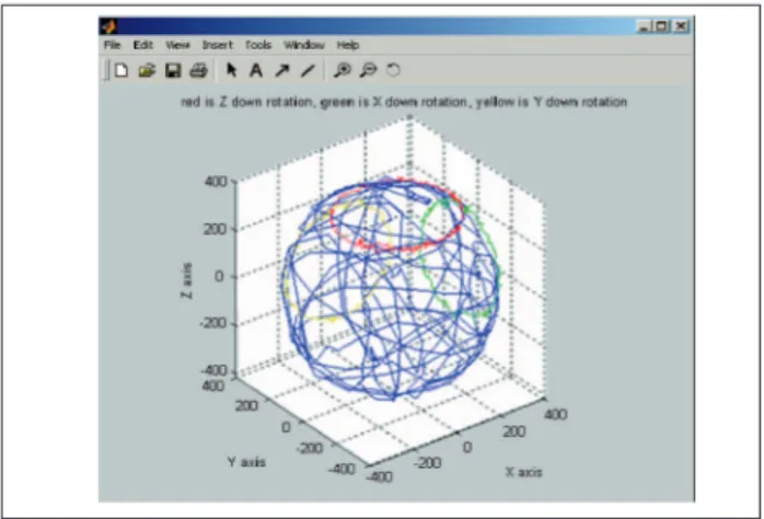
he experimental tests used a CubeSat mockup built to provide three-axis movements (X, Y and Z axis of the body coordinates frame). he CubeSat body is composed of transparent acrylic polyethylene plates, a system of bearings, and supports for the Arduino platform and for the magnetometer HMC5843. Figure 3 shows the CubeSat mockup.
Figure 3. The CubeSat mockup for experimental tests of magnetometer calibration.
–300
–300
–200 200 300
–200 0 200 300 By
[mG]
Bx [mG]
–300
–300
–200 200 300
–200 0 200 300 Bz
[mG]
Bx [mG]
–300
–300
–200 200 300
–200 0 200 300 Bz
[mG]
By [mG] SATELLITE MANEUVERS FOR MAGNETIC DATA
ACQUISITION
he tests of magnetometer calibration use single mockup rotations around the three axes of the body coordinates frame (X, Y, Z), as can be seen in Fig. 4. he rotations are manually
Figure 4. Two maneuvers of the CubeSat mockup for magnetometer data acquisition: rotation around one axis and aleatory motion.
performed, without strict control of rapidity or duration of the motion, because these parameters are not important in the calibration tests. he calibration can also be done using aleatory motion combining rotations around all axes (Fig. 4).
TESTS RESULTS
TESTS OF THE GEOMETRIC CALIBRATION APPROACH
The geometric method is applied for experimental tridimensional calibration of the magnetometer HMC5843. he experimental procedure consists of rotation of the satellite mockup around the three axes of magnetometer frame. he irst rotation is around the Z axis, the second one, around Y axis, and the last rotation, around X axis. he resulting magnetic ield measurements are shown in Fig. 5.
he results of parameters calculation for the calibration are shown in Table 1.
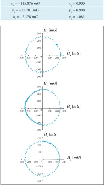
Table 1. Results of calibration process by geometric method.
bx = –115.876 mG xsf = 0.935
by = –27.701 mG ysf = 0.998
bx = –2.178 mG zsf = 1.081
–300
–300
–200 –100 100 300
–200
0 200
–100 200
100 300 Hy
[mG]
Hx [mG]
–300
–300
–200 –100 100 300
–200
0 200
–100 200
100 300 Hz
[mG]
Hx [mG]
–300
–300
–200 –100 100 300
–200
0 200
–100 200
100 300 Hz
[mG]
Hy [mG]
ˆ ˆ
ˆ ˆ
ˆ
ˆ
Figure 6. The graphics of Hx, Hyand Hz measurements of the sensor HMC5843 after calibration using 3-D geometric method.
Figure 6 shows the graphics of Hx, Hy and Hz measurements, obtained by the magnetometer HMC5843, calibrated by the geometric method applied to three-dimensions problem.
In the irst step of TWOSTEP algorithm, the results are:
TESTS OF THE TWOSTEP ALGORITHM
The first tests using TWOSTEP calibration algorithm comprehended numerical simulations using a CubeSat lying in typical orbit, with stabilized attitude keeping the X axis pointed to the Sun, and considering a simulated noise disturbing the magnetometer HMC5843 of magnitude σ0 = 2.8 mG per axis. he resulting simulated geomagnetic ield is shown in Fig. 7.
k
B
[
mG
]
400,000
200,000
0,000
-200,000
-400,000 1 25 49 73 97
121 145 169 193 217 241 266 289 313 337 361 385 408 433 457 481 506 529 553 577 601 625 649 673 687
Bx
By
Bz
Figure 7. Simulated measurements of the geomagnetic ield for the magnetometer calibration procedure, with X axis of satellite pointed to the Sun.
he centralized Fisher information matrix is then obtained:
And the Fisher information matrix for the central value correction is given by:
he resulting factor is c = 2.604. In this case, where the satellite is stabilized, the error vector components are less observable. Consequently, the estimation of the systematic error obtained in the second step of the algorithm (see details of the iterations in Table 2) is:
A second case for numerical simulation of the calibration
^ ^ ^
(36)
(37)
(38)
(39)
procedure considers the same noise disturbing the magnetometer HMC5843, i.e. the magnitude per axis. But now the satellite keeps the Z axis pointed to the center of the Earth. he resulting simulated geomagnetic ield is shown in Fig. 8.
Figure 8. Simulated measurements of the geomagnetic ield for the magnetometer calibration procedure, with Z axis of satellite pointed to the center of the Earth.
Table 2. Results of iterations of the second step of the algorithm (σ0 = 2.8 mG, satellite stabilized, axis X pointing to the Sun).
Iteration bix biy biz
0 −16.966 −36.478 12.007
1 −17.361 −36.809 11.997
2 −17.361 −36.809 11.997
k
B
[
mG
]
400,000
200,000
0,000
-200,000
-400,000 1 25 49 73 97
121 145 169 193 217 241 266 289 313 337 361 385 408 433 457 481 506 529 553 577 601 625 649 673 687
Bx
By
Bz
In the irst step of TWOSTEP algorithm, the results are:
One can remark that σv02 is bigger than the precedent case.
he vector b tends to be more distant from the magnitude of the geomagnetic ield vector.
he centralized Fisher information matrix is then obtained:
And the Fisher information matrix for the central value correction is given by:
In this case, the resulting factor is c = 18.527. Again, with the satellite body stabilized, the error vector components are weakly observable. The estimation of the systematic error obtained in the second step of the algorithm (see details of the iterations in Table 3) is:
Iteration bix biy biz
0 −15.763 −37.764 11.679
1 −16.790 −37.189 11.882
2 −16.787 −37.189 11.881
Table 3. Results of the second step of the algorithm (σ0 = 2.8 mG, satellite stabilized, axis Y pointing to the center of the Earth).
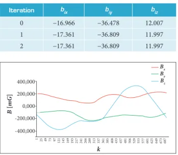
he experimental magnetometer calibration was performed using the algorithm TWOSTEP embedded in the satellite mockup. he main supposition for the tests is that the geomagnetic ield is constant for a ixed point and for a short time period. his is not the case for a satellite orbiting the Earth at a high displacement speed. Meanwhile, the main purpose of these tests is to verify the performance of the calibration algorithm to ilter noises in the magnetic ield measurement. he results shown in Fig. 9 are related to data acquisition during aleatory maneuvers as illustrated in Fig. 4. Considering the calculations of the irst step of TWOSTEP algorithm, the results are:
(40)
(44)
(41)
(45) (42)
(43)
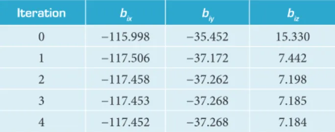
Iteration bix biy biz
0 −115.998 −35.452 15.330
1 −117.506 −37.172 7.442
2 −117.458 −37.262 7.198
3 −117.453 −37.268 7.185
4 −117.452 −37.268 7.184
Table 4. Results of the second step of the algorithm. k
B
[
mG
]
300,000
100,000
-100,000
-300,000
1 25 49 73 97
121 145 169 193 217 241 266 289 313 337 361 385 408 433 457 481 506 529 553 577 601 625 649 673 687
Bx
By
Bz
Figure 9. Earth magnetic ield measurements by the magnetometer embedded in the CubeSat mockup.
For the centralized value correction, the Fisher matrix is calculated:
In this case, the proportion factor is c = 0.696. It means that the second step of the calibration algorithm must continue. he estimation of systematic error with the centralized correction calculated ater four iterations (the details of the iterations results are shown in Table 4) of the second step is:
use of noisy data measured by magnetometer HMC5843 made the central values obtained in step two stay slightly outside the expected range. his leads to the need for investing in better magnetometers in order to improve the accuracy of the results.
As shown by simulations, the TWOSTEP algorithm works well in all phases of spaceship operation, especially in the case of artificial satellites, from the orbit injection phase, with the spacecraft spinning, to the moment when the ship has its attitude completely stabilized (with the Z axis, simulating the load direction, pointing to the Earth). The systematic error vector (bias) components are more observable when the Earth’s magnetic field vector is changing regularly. Therefore, the best time to measure the systematic error is immediately after the orbit injection when the satellite is still spinning. In the tests, the worst time is when the satellite is fully stabilized, with its Z axis pointing to the Earth, when the components vary slightly.
The simulations also show that, for a spaceship in a geostationary orbit, with the attitude stabilized, the TWOSTEP algorithm will not converge. he estimate of the systematic error of the measured value tends to the magnetic ield vector in this particular case.
CONCLUSION
This project presented a review and an experimental implementation of methods for magnetic ield sensor calibration in the context of an embedded device for applications in vehicle navigation systems like artiicial satellites. he Arduino MEGA 2560 was perfectly capable of performing the most complex mathematical calculations required by the geometric method. his method requires absolute attitude control during calibration. It also applies most commonly to small devices and vehicles. It is not ruled out, however, the need to recalibrate the magnetometer during the mission, using other methods. he test results showed that TWOSTEP algorithm is fast and robust in the calculation of the bias magnetic field vector. his method, despite the simplicity of the equations, requires accumulation of data to calculate some parameters preliminarily. herefore, the primary bias was estimated from the irst batch of magnetometer measurements.
Comparing these two implemented methods of calibration, it can be seen that all are fast and reach the desired results, with comparable estimates. However, the navigation system, (46)
(47)
In general, it appears that the use of a noisy magnetometer makes the results show less precisely in relation to those obtained by Alonso and Shuster (2002). In the case where the satellite is stabilized, with Z axis pointing to the Earth, it can be noted that the measurements of the Y axis of the magnetic ield vector are hardly observable, even ater the application of step two. his can be seen in Fig. 8, where there is little variation in the measured values.
the mission, and especially the device or vehicle will determine which magnetometer calibration method is the most applicable in each case, including the possibility of using a combination of methods.
ACKNOWLEDGEMENTS
he authors acknowledge the institutional support of the Universidade Federal do ABC (Brazil).
REFERENCES
Alonso R, Shuster MD (2002) TWOSTEP: a fast robust algorithm for attitude-independent magnetometer-bias determination. J Astronaut Sci 50(4):433-451.
Alonso R, Shuster MD (2003) Centering and observability in attitude-independent magnetometer-bias determination. J Astronaut Sci 51(2):133-141.
Arduino (2005) Smart Projects, Ivrea, Italy; [accessed 2012 Feb 14]. www.arduino.cc
Caruso MJ (2000) “Applications of magnetic sensors for low cost compass systems. Proceedings of the IEEE on Position Location and Navigation Symposium, San Diego, USA.
Crassidis JL, Lai KL, Harman RR (2005) Real-time attitude-independent three-axis magnetometer calibration. J Guid Contr Dynam 28(1):115-120.
Honeywell (2009) HMC5843 3-axis digital compass IC. Honeywell Inc., Morristown, NJ, 1-19; [accessed 2012 Feb 14]. www.honeywell.com
Inamori T, Nakasuka S (2012) Application of magnetic sensors to nano- and micro-satellite attitude control systems. In: Kuang K, editor.
Magnetic sensors: principles and applications. Rijeka, Croatia: InTech. p. 85-102.
Juang JC, Tsai YF, Tsai CT (2012) Design and veriication of a magnetometer-based orbit determination and sensor calibration algorithm. Aero Sci Tech 21(1):47-54. doi: 10.1016/ j.ast.2011.05.003
Kim E, Bang HC (2007) Bias estimation of magnetometer using genetic algorithm. Proceedings of the International Conference on Control, Automation and Systems; Seul, Korea.
Pisacane VL (2005) Fundamentals of space systems. New York: Oxford University Press.
ST Microelectronics (2012) AN3192 application note: using LSM303DLH for a tilt compensated electronic compass; [accessed 2012 Apr 17]. www.st.com
![Figure 3. The CubeSat mockup for experimental tests of magnetometer calibration. –300 –300–200 200 300–2000200300By [mG] B x [ mG ] –300 –300–200 200 300–2000200300Bz [mG] B x [ mG ] –300 –300–200 200 300–2000200300Bz [mG] B y [ mG ]SATELLITE MANEUVERS](https://thumb-eu.123doks.com/thumbv2/123dok_br/18889830.424749/6.926.479.824.548.1062/figure-cubesat-mockup-experimental-magnetometer-calibration-satellite-maneuvers.webp)