Abstract—Fiber Bragg gratings (FBGs) offer new possibilities to monitor accurately the rotor temperature. Dozens of sensors can be mounted in series in a single fiber and used to measure the temperature in several points of the rotor winding. Such sensors installed directly on the rotor winding surface are thermally isolated from the cooling air by a silicone layer. Because of the temperature gradient in this structure, the sensor is exposed to thermo-mechanical stresses and therefore can be deformed. Since the FBG probes are sensitive to both temperature and strain, the knowledge of each effect separately is necessary to ensure that the temperature readings are not affected by strain. Experimental results obtained in rotor winding mockup tests with thermistors and FBG sensors show that the temperature readings by the FBG are 4.5°C above the temperature defined by the thermistors which were used as references. Multi-physics simulations were carried out to calculate the strain and temperature in the FBG assembly. The theoretical and experimental results are in a good agreement.
Index Terms—Hydro generator, rotor, fiber Bragg grating, temperature measurement.
I. INTRODUCTION
During normal operation, the rotor is exposed to thermal and mechanical stresses. Above some acceptable limits these factors lead to premature aging of the rotor. Thermal stress normally affects the turn and ground insulation of the rotor poles [1]-[3]. This may lead to early refurbishment of the poles or in some cases to ground faults which can cause extensive damage.
Continuous monitoring of temperature of the field winding (rotor winding on synchronous machines) could provide early warning of accelerated aging due to abnormal temperatures and improve reliability of the equipment by proper condition based maintenance. However, measurement of temperature in several locations (e.g. field windings and pole connections) is not a trivial task. Such procedure was avoided in the past due to issues related to cost, reliability, difficulty of instrumentation and signal extraction [3],[5].
A common way to determine the rotor temperature is to measure the winding resistance and calibrate it to copper temperature change, but this method gives only an average temperature and does not address the problem
Analysis of Thermo-Mechanical Stress in
Fiber Bragg Grating
Used for Hydro-
Generator Rotor Temperature Monitoring
R.C. Leite¹, V.Dmitriev²¹Technological Centre of Technology of Eltrobras Eletronorte, Belém, Pará, Brasil. ²Federal University of Pará, Belém, Pará, Brasil
e-mails: [email protected], [email protected]
C.Hudon³, S.Gingras³, C.Guddemi³,J.Piccard³, L.Mydlarsky4
³Institut de Recherche d'Hydro-Québec, Varennes, Québec, Canada,
4
McGill University, Montréal, Québec, Canada
of hot spots. Point sensors (thermo-couples) were used in the past for rotor temperature monitoring, but the signal retrieval is not obvious and this requires installing long conductive wires on the rotor which rises long term safety concerns [2]. Another available monitoring method is to insert an infrared (IR) probe through a vent duct in the stator to measure the temperature of the poles passing in front of the probe. However it does not define the hot spots of the field winding and the measurement depends on the emissivity of the pole surface which is not always known and can be affected by contamination [3].
To overcome these problems of the temperature monitoring, the systems using Fiber Bragg Grating (FBG) optical sensors were proposed. FBGs are used in power generators to monitor either the stator and the rotor. In [7] the FBG were installed behind each radiator around the stator winding for temperature monitoring Another use of FBGs in hydro-generators is exposed in [4] and [8] where a system that monitors rotor temperature and displacement using FBG sensors based on a interrogator that permits the visualization of the spectrum signal from the sensors is suggested. Two collimators, one fixed on the rotor and other fixed on the stator, extract the measurement data from the rotor to the monitoring system. In [5], a system that monitors the rotor temperature by means of an array of FBG sensors in conjunction with a rotary joint was proposed. Some care must be taken when installing the FBG sensors on the rotor because of the high centrifugal force acting radially in the rotor [9]. The sensors are usually glued to the rotor winding using a thermal adhesive and covered with a epoxy silicone layer to insulate from the cooling air and protect against the pollution of the rotor environment.
Unlike FBG sensors traditional installations (embedded in structures of bridges, dams, tunnels, etc) where the influence of external disturbances such as the thermal gradient across the installation are avoided [6], the FBG sensors used for rotor temperature monitoring installed at rotor pole surface form a three layer composite. One of the composite is a thermal adhesive to fix the sensor to winding surface, the sensor itself with its packaging and an additional protective silicone layer. This assembly is situated in a temperature gradient between the hot spot of the rotor copper and the adjacent cooling air. This means that the thermal stresses present during normal rotor operation can deform the materials and this can cause a bending of the sensor. The bending can induce an axial stress on the FBG sensor and since these sensors are sensitive to both axial stress and temperature [10]-[13], the rotor temperature readings can lead to erroneous results.
In this work, we study the effects of thermo-mechanical stresses in a FBG sensor assembly. The experimental part of the work is based on laboratory tests where the assembly is installed on the rotor winding. The numerical multi-physics simulations using the Finite Element Method (FEM) and experimental results are compared and discussed.
II. LABORATORY TESTS
A. The rotor winding mockup
Fig. 1. Polar coil, adapted from [1].
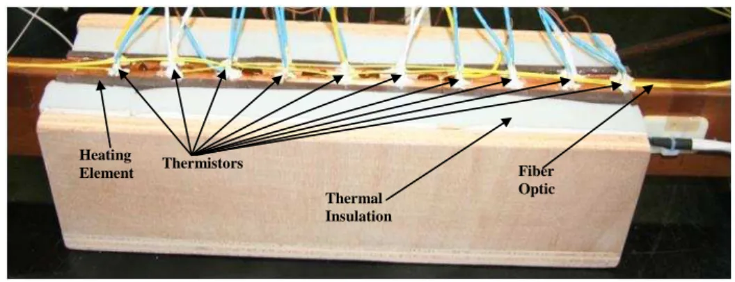
The rotor winding mockup simulates two turns of these coils and the way the FBG sensors would be installed on the actual rotor winding. This setup is formed by two copper bars with dimensions of 610 x 80 x 5 mm each separated by a thermal insulating sheet of NOMEX. On the sides of each bars the thermal elements are installed to provide a heat flux on each bar surface in order to heat them uniformly, simulating the heating from DC current flow as in the generator winding. The reference temperature is obtained by fixing the power which provides the desired temperature level. Fig. 2 shows the rotor winding mockup.
Heating
Element Thermistors Fiber
Optic Thermal
Insulation
Fig. 2 - Rotor winding mockup.
Ten thermistors were installed in the holes of 2 to 3 mm deep on the edge of each bar and labeled from 1 to 10 in one of the bars and from 11 to 20 in the other one. As the FBG sensor is installed at the center position of the bars, the average temperature of the thermistors around the FBG probes was used as temperature reference for their readings.
B. The rotor winding mockup tests
The test on the rotor winding mockup consisted in temperature measurements in the five assigned
temperature levels in the two ways: the first one was accomplished during the copper bar heating
process. The assigned temperature level was reached during 10 min stabilization time order to attain
the thermal equilibrium. This process was repeated up to the maximum assigned level. The second
temperature measurement was carried out during the cooling process, which was fulfilled by using a
fan to provide the air flux necessary to cool the setup and adjusting the power of the heating elements.
TABLE I. ASSIGNED TEMPERATURE LEVELS
Process Temperature levels (°C)
Heating 40; 60; 80; 100 Cooling 80; 60; 40
C. The rotor winding mockup test results
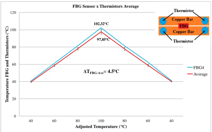
The ordinates in Fig. 3 corresponds to the temperature readings of the FBG sensor and the average of the thermistors readings at the center position of the bars. The abscises are the temperatures of the predetermined assigned set point for a complete cycle of heating (see Table I) and of cooling back down to 40°C. The inset in Fig. 3 shows the position of the FBG sensor relative to the thermistors.
102,32C
97,85C
0 20 40 60 80 100 120
40 60 80 100 80 60 40
T
em
p
er
a
tu
re
F
B
G
a
n
d
Th
er
m
is
to
rs
(
C)
Adjusted Temperature (C) FBG Sensor x Thermistors Average
FBG4 Average
ΔTFBG-Ave= 4.5C
Fig. 3 - Comparison between FBG sensor readings and thermistors average at the center location.
It can be seen from Fig. 3 that the difference between the FBG sensor and the thermistors readings
increases with the copper bar temperature, reaching a maximum of 4,5°C at 100°C. Also it can be
noticed that the FBG temperature is higher than the thermistors readings, which is an unexpected
result, since the thermistors are in direct contact with the copper and the FBG has a thermal adhesive
between it and the copper. According to [14], it increases the thermal resistance and should give a
reading temperature smaller than the one on the copper bar. Such a difference could be due to one of
the following causes: (1) effect of copper thermal expansion in the axial direction. If the copper bars
expand with the sensor fixed on them, they can provoke a mechanical stress in the axial direction of
the FBG sensor which would induce false readings due to its strain sensitivity; (2) a bad thermistors
installation used as reference, causing poor contact between copper and the probe; and (3) effect of a
temperature gradient across the sensor installation, i. e. while the rotor winding mockup is at a fixed
cause unequal expansion of the materials that compose the sensor installation and could cause
bending as shown in in the bottom part of Fig. 4.
Fig. 4 - FBG sensor deformation due to temperature gradient. When the gradient is 0 there is no deformation, when the temperature gradient is different from zero, the sensor will deform.
In order to test the hypothesis on the previous paragraph, the rotor winding mockup was put in an
oven. The idea was to provide an environment where the rotor winding mockup and the copper bar
was at the thermal equilibrium eliminating the temperature gradient between the top and the bottom of
the FBG installation assembly. The first graph (Fig. 5a) shows the results for the rotor winding
mockup when it was heated in the oven at 100°C and the second one shows the results for the rotor
winding mockup heated by the heating elements (Fig. 5b). It can be seen from these figures that the
difference between readings of FBG sensors and the thermistors is smaller (less the 1°C) when the
whole setup is heated in the oven in comparison with the case when the setup is heated by heating
elements (around 5°C).
This analysis leads to the conclusion that the thermistors provide the the correct reading of
temperature. Therefore, the above mentioned hypothesis (1) and (2) can be rejected. The thermal
expansion effect can be discarded because if this hypothesis was true, the same difference should
appear again when the rotor winding mockup was heated by the oven.This leaves hypothesis (3) to be
tested.
Δ
T = 0
95 96 97 98 99 100 101 102 103 104
13:39 13:39 13:39 13:39 13:39 13:39 13:39
T
em
p
er
a
tu
re
(
C)
Tempo (h:mm)
Temperature Difference Between FBG and Thermistors
FBG4(Micron)
Thermistance Average
(a)
95 96 97 98 99 100 101 102 103 104
13:37 13:37 13:37 13:37 13:37 13:37 13:37
T
em
p
er
a
tu
re
(
C)
Tempo (h:mm)
Temperature Difference Between FBG and Thermistors
FBG4
Thermistance Average
(b)
Fig. 5 - (a) Temperature difference between FBG sensors readings and thermistors average when rotor winding mockup was heated in the oven. (b) Temperature difference between FBG sensors readings and thermistors average when rotor winding
mockup was heated by the thermal elements.
The next step in the research was to investigate the effect of a temperature gradient on the sensor
assembly. For this a thermo-mechanical model of the sensor assembly was developed and numerical
III. FBG THERMO-MECHANICAL MODEL
A thermo-mechanical model was used to understand how the temperature gradient can influence the
FBG sensor readings. The problem is to calculate the temperature in the fiber core, which is the
sensing portion of the fiber, and also the deformation and strain caused by the temperature gradient
across the sensor assembly. The results obtained from this model were used to feed the optical model
and to calculate the modifications in the refractive index and in the grating period. This allows one
analyze the shift in the Bragg wavelength.
A. Thermo-Mechanical Model
The thermal stress across the sensor assembly was numerically calculated by using the COMSOL
Multiphysics software that is based on the Finite Element Method. The calculation was carried out in
two steps: first the temperature across the model was determined by using the software Heat Transfer
interface and then the thermal stress was calculated by using the Thermal Stress Interface from the
Structural Mechanics Module [15]. The result was then converted in wavelength shifts using Optical
model described further. The optical temperature sensor based on FBG has a cylindrical shape. It is
composed by an optical fiber embedded in a protection housing, the optical fiber is made of fused
silica and has a core of 8.2mm and a cladding 125mm [16],[17]. An alumina housing is mounted
around the fiber to provide protection and mechanical decoupling.
For the traditional FBG applications this housing would be a sufficient protection, but in the harsh
environment of a hydro-generator this kind of protection is not enough. As stated before the rotor is
exposed to strong mechanical forces and thermal stresses [9] and as the sensor is to be installed on
outer turns of the rotor windings, it will be submitted to the same stresses. So to avoid the sensor to
detach from the rotor by the centrifugal force, it was mounted over a bed of thermal adhesive to
provide a better thermal contact with copper conductors and to keep the sensor attached to the field
winding.
A silicone layer completes the assembly and its function is to reduce the effect of the convective
heat loss from the cooling fluid (air) which flows around the sensor [18]. The 3D model geometry is
shown in Fig. 7, the problem was treated with a mesh composed of 43160 free tetrahedral elements of
the following types domain elements, 10.968 boundary elements and 1201 edge elements, these
elements are well defined on [19], Fig. 8 shows the model with the mesh. This figure provides also
the type of materials used in the sensor installation. The sensor presents a three layer composite. The
bottom part of the assembly which is in contact with the copper representing the field winding, is the
Fig. 6 - FBG sensor thermo-mechanical model.
Fig. 7 - Mesh applied to the FBG thermo-mechanical model.
The heat will be conducted from the copper conductor through the adhesive and then through the
sensor housing until it reaches the fiber core. The heat will then be conducted through the silicone
layer to the top of the model. Fig. 8 shows a sketch of the cross-section of the sensor installation and
Fig. 8 – Cross-section showing the sensor installation and the heat flux.
This process is governed by equation (1), where ρ is the density (kg/m³); cp is the specific heat
capacity; u is the velocity vector; T is the absolute temperature; k is the thermal conductivity; Q is the
power density, that in this study is zero.
Q T) .(k T
cp.u .
. (1)
From this point the thermal energy will be conveyed by natural convection to the air and is decribed
by equations (2) and (3) below.
0
q
n q . (2)
Equation (2) represents a specified heat flux boundary condition where q is conductive heat flux
vector; n is the unit normal vector at the boundary and q0 is the heat flux normal to the boundary [15].
There are two boundary conditions of this type, the first one is a special case called thermal insulation
boundary condition where q0 is zero and in this case n·q=0 [15]. The other boundary condition of
prescribed flux used in this model is a common type where the normal heat flux q0 flowing through
the surface and is given by equation (3) [20]:
) (
0 hT T
q ext , (3)
where h is the local convection coefficient, Text is the temperature of the fluid that surrounds the
surfaces and T is the surface temperature (K). This boundary condition represents the heat transfer by
natural convection that occurs at the top of the model with a convection heat transfer coefficient of
17.57 W/m²K for the fluid cooling the surface. The mechanical behavior of model is modeled by a
multi-physics coupling of the thermal expansion given by Equation (4) ([15],[20]):
r ef
th TT
, (4)
where α is thermal expansion coefficient, T is the temperature and Tref is the temperature when the
body has no deformation.
The optical model represents the FBG sensoring function. These sensors act like mirrors reflecting
specific wavelengths that obey the resonance condition given by ([5]-[8]):
eff
B 2 n
where λB is the Bragg wavelength, neff is effective refraction index and Λ is the grating period. The
FBGs are sensitive to strain and temperature and due to this feature they can be used as distributed
sensor network where several sensors are inscribed along the fiber giving point readings of the
variables described above. The strain or temperature are measured according to the shift of the Bragg
wavelength caused by the modification of the refractive index or the grating period due to the
elasto-optic effect and fiber deformation due to stress or thermo-elasto-optic effect or fiber thermal expansion for
the temperature [10]-[14]. Equation (6) is used to model all the effects:
T dt dn n P P P n n B 1 2 12 12 11 12
2
, (6)
where DlB is the shift on Bragg wavelength, n is the refraction index, L is the grating period, Pij are
the Poeckels coefficients, n is the Poisson ratio, ε is the strain, α is the thermal expansion
coefficient and DT is temperature variation.
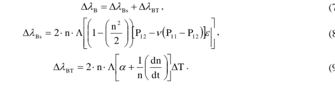
It can be easily seen from equation (5) that the Bragg wavelength shift can be rewritten as follows:
BT Bs
B
, (7)
12 11 12
2
2 1
2 n n P P P
Bs , (8)
T dt dn n n
BT
2 1 . (9)
The values of temperature variation and strain are obtained from the numerical simulation of the
thermo-mechanical model and used in Equations (8) and (9) to calculate the shift of the Bragg
wavelength due temperature (DlBT) and strain (DlBS). Notice that equation (7) gives the total shift of
the Bragg wavelength.
The next step is to calculate the new Bragg wavelength (lB1) using equation:
B B
B
1 . (10)
B. Simulation Results for the Rotor winding mockup
Fig. 9 shows a temperature gradient of 17.7°C observed between the top (right hand side of the
graph) and the bottom (left part of the curve) of the assembly (thermal adhesive + FBG + silicone)
modeled in this graph. This temperature difference occurs due to the thermal stress acting on the FBG
sensor. As the temperature gradient across the sensor assembly increases, the thermal stress increases
two, Equation (4) in the text shows that the thermal stress is directly proportional to temperature
gradient. The thermal stress appears due to the assembly bending caused by the different coefficients
temperature and strain changes, the effects of temperature and strain add and cause this difference in
temperature readings. This effect was observed during the tests in the field winding mock up.
The impact on actual measurements will occur due to the fact that when the sensors are installed
on the generator rotor there will be a temperature gradient between the field winding surface and the
air circulating inside the generator. If this gradient is high enough to cause the assembly bending, this
could make the sensor reads a temperature value greater than the actual one and lead to wrong a
decision, stopping the machine unnecessarily for instance.
The circle in Figure 9 shows where the FBG sensor is located. When the copper temperature is
100°C, the calculated temperature at the core of the fiber of 98.9°C, without any contribution of the
strain in this calculation, as shown in Fig. 9. It should be pointed out that the actual FBG temperature
reading in this condition (100.0°C set point, and natural convection) was of 102.3°C (in the mockup).
Thus the FBG temperature calculated in the model is 3.4 °C below the actual temperature read by the
FBG. This difference is very close to the 4.5 °C recorded between the FBG readings and the
thermistors average found in the mockup at 100.0°C.
Fig. 9 - Temperature measured along the diameter of the sensor assembly.
Table II shows the strain calculated by the thermo-mechanical model that shows that the actual
strain increases with bending as the temperature increases. The shift in the Bragg wavelength can be
determined by inserting the values displayed in Table II into Equation 8. Thermal
Adhesive
FBG Sensor Housing
Silicone
Tcu = 100°C TFBG = 102,3°C
TABLE II. STRAIN CALCULATED ALONG SENSOR AXIS
Setpoint Temperature
(°C)
Strain (10-5ε)
40 1.65 60 3.31 80 4.99 100 6.50
The value of DlB was used in Equation (11) that was provided by the sensor manufacturer [21] to
calculate the temperature. The results of this correction are shown in Table III. It can be seen by the
tabulated results that the temperature value reading by the FBG sensor is very close to that obtained
by the optical model when the strain produced by the temperature gradient is considered. If the strain
value is disregarded on Equations (6) and (8), the temperature calculated by the optical model stays
close to the temperature calculated by FEM on the thermo-mechanical model.
TC33 C22 C1C0
where T is the temperature in (°C), l is the wavelength calculated from Equation (10) in (nm), C1,C2
and C3 are constants unique for each sensor listed on Table IV.
TABLE III. COMPARISON BETWEEN TEMPERATURE WITH AND WITHOUT STRAIN EFFECT
FBG Measured Temperature
in mockup (°C)
Optical Model Temperature
with ε (°C)
Optical Model Temperature
without ε (°C)
Thermo-mechanical Model Temperature
(°C)
40.6 40.58 38.5 39.8
61.0 61.78 57.9 59.6
81.5 82.13 76.5 79.3
102.3 103.15 96.7 98.5
TABLE IV.FBG SENSOR CONSTANTS
Constant Value
C3 4.1398095
C2 -18,843.31
C1 28,589,998
C0 3.8686
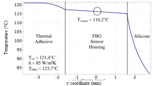
The next step was to simulate the FBG assembly behavior for an actual generator winding where a
temperature of 121.4°C was imposed as the field winding temperature as the Dirichlet boundary
condition. This temperature was estimated by taking the readings of an actual FBG sensor (123.7°C in
average) installed on a Hydro-Québec generator as described in [5] from which was subtracted 2.3°C
from it. This value of 2.3°C was obtained from the experiments on the rotor winding mockup which
shown that in average the FBG temperature was slightly higher than the actual copper temperature by
this value.
The temperature difference was determined by the tests carried out on the rotor winding mockup
and described in Section II. In this case, the forced convection process of the generators with radial
cooling through rim ducts was considered and simulated using the local convection coefficient h
around the field winding conductor of 85 W/m² determined in [22]. Figure 10 shows that in such
conditions, a 35°C gradient builds up across the FBG sensor assembly.
Fig. 10 - Temperature distribution along the model diameter.
The temperature at fiber core (FBG sensor) calculated by the model without strain effect is of
116.2°C, while the temperature reading by the actual FBG on the generator was of 123.7°C. A strain
of 4.99x10⁻⁵ was calculated by the model under the conditions described above. The same strain
correction as before was analysed in the optical model and the results are presented in Table V. This
Table compares the temperatures measured by the FBG sensors installed on the generator with that
calculated by the optical model with and without strain and compares the temperature between the
optical model without strain and the thermo-mechanical model (two last columns in Table V).
When the strain is added to the optical model there is an increase of about 6°C in the calculated
reading of the FBG (second column in the Table V), so the mechanical decoupling of the FBG is not
perfect. However, since the active part of the sensor is in indirect contact with the copper surface its
reading is lower than the actual hotspot, but this difference was almost perfectly compensated by the
strain from the bending of the FBG assembly. This resulted in a measured temperature on the
generator (first column) similar to the calculated one. It can be seen from these results that the
difference is negligible.
Thermal Adhesive
FBG Sensor Housing
Silicone
Tcu = 121,4°C h = 85 W/m²K TFBG = 123,7°C
TABLE V. COMPARISON BETWEEN TEMPERATURE WITH AND WITHOUT STRAIN AT THE GENERATOR
FBG Measured Temperature
on the generator
(°C)
Optical Model Temperature
with ε (°C)
Optical Model Temperature
without ε (°C)
Thermo-mechanical
Model Temperature
(°C)
123.7 124.8 118.5 116.7
IV. CONCLUSION
We studied in this paper influence of the temperature gradient across the different
materials that compose an FBG sensor assembly on its readings. Experimental tests in a field
winding experimental set-up were performed and the difference of 4.5°C was found between
the FBG and the thermistor readings used as references. A thermo-mechanical multiphysics
model of the FBG assembly placed on the field winding was used to calculate the axial strain
in the sensor. The results of the model simulations agreed with experimental results and
showed that the bending caused by the silicone layer of the sensor produces an axial strain.
This strain is responsible for the change in the FBG reading. Our future work will be focused
on the optimization of the sensor structure in order to minimize the error in the FBG
readings.
ACKNOWLEDGMENT
R. C. Leite gratefully acknowledge CNPq and Eletrobras for the scholarship of the Science
Without Borders program and IREQ - Institut de Recherche d'Hydro Québec for having me as guest
researcher and granting access to its laboratories and facilities.
REFERENCES
[1] Hemery, G. (2008). Alternateurs Hydrauliques et compensateurs. Ed. Techiniques Ingénieurs.
[2] Stone, G. C. (2013). Condition monitoring and diagnostics of motor and stator windings–A review. IEEE Transactions on Dielectrics and Electrical Insulation, 20(6), 2073-2080.
[3] Hudon, C., Lévesque, M., Torriano, F., Gingras, S., Picard, J., & Petit, A. (2014, June). On-line rotor temperature measurements. In 2014 IEEE Electrical Insulation Conference (EIC) (pp. 373-377). IEEE.
[4] Rosolem, J. B., Floridia, C., Dini, D. C., Hortencio, C. A., Borin, F., Neto, J. B. D. M. A. & Sanz, J. P. M. (2010). Tecnologias de monitoração de hidrogeradores utilizando sensores ópticos. Cad. CPqD Tecnologia, 6(1), 21-30.
[5] C. Hudon, S. Gingras, C. Guddemi, L. Mylarski and R. C. Leite. Rotor temperature monitoring using Fiber Bragg Gratings. In IEEE Electrical Insulation Conference (EIC)(pp. 456-459), IEEE
[6] Dreyer, U., Sousa, K. D. M., Somenzi, J., Lourenço Junior, I. D., Silva, J. C. C. D., Oliveira, V. D., & Kalinowski, H. J. (2013). A technique to package Fiber Bragg Grating Sensors for Strain and Temperature Measurements.Journal of Microwaves, Optoelectronics and Electromagnetic Applications,12(2), 638-646.
[7] Allil, R. C. S. B., Werneck, M. M., Ribeiro, B. A., & de Nazaré, F. V. (2013). Application of fiber Bragg grating sensors in power industry. Current Trends in Short-and Long-Period Fiber Gratings, 133-166.
[8] Floridia, C., Rosolem, J. B., Borin, F., Bezerra, E. W., & Said, J. C. (2009, October). Asynchronous FBG interrogation system for temperature and strain monitoring on hydrogenerator rotors. In 20th International Conference on Optical Fibre Sensors (pp. 75033I-75033I). International Society for Optics and Photonics.
[10]Hill, K. O., & Meltz, G. (1997). Fiber Bragg grating technology fundamentals and overview. Journal of lightwave technology, 15(8), 1263-1276.
[11]Othonos, A. (1997). Fiber bragg gratings. Review of scientific instruments,68(12), 4309-4341.
[12]Rao, Y. J. (1999). Recent progress in applications of in-fibre Bragg grating sensors. Optics and lasers in Engineering, 31(4), 297-324.
[13] Kersey, A. D., Davis, M. A., Patrick, H. J., LeBlanc, M., Koo, K. P., Askins, C. G., ... & Friebele, E. J. (1997). Fiber grating sensors. Journal of lightwave technology, 15(8), 1442-1463.
[14]Giallorenzi, T. G., Bucaro, J. A., Dandridge, A., Sigel, G. H., Cole, J. H., Rashleigh, S. C., & Priest, R. G. (1982). Optical fiber sensor technology.IEEE transactions on microwave theory and techniques, 30(4), 472-511.
[15]COMSOL Multiphysics, Heat transfer module user's guide, October 2014.
[16]Jackson, J. D. (1999). Classical electrodynamics. Wiley..
[17]PI1036; Corning SMF -28, Single Mode Optical Fiber, Product information, April 2002.
[18]M. Chaaban, M. Lessard, "Analyse numérique et expérimentale de l'erreur potentielle commise lors de la mesure de témperature de surface," Institut de Recherche d'Hydro-Québec - IREQ, Montreal, QC, Canada, Jan. 2011.
[19]COMSOL Multiphysics, Reference Manual, October 2014.
[20]Bergman, T. L., Incropera, F. P., DeWitt, D. P., & Lavine, A. S. (2011).Fundamentals of heat and mass transfer. John Wiley & Sons.
[21]MICRON OPTICS Inc, Grating Based Temperature Sensors - temperature calibration and thermal response, November 2008, retrieved from http://www.micronoptics.com/download/grating-based-temperature-sensors-temperature-calibration-and-thermal-response.