Nonlinear dynamic behavior and instability of slender frames with semi-rigid connections

(1)

Nonlinear dynamic behavior and instability of slender frames

with semi-rigid connections

Alexandre S. Galv

ao

~

a

, Andre´a R.D. Silva

b

, Ricardo A.M. Silveira

b

, Paulo B. Gonc

-

alves

c,n a_{Universidade Federal Fluminense, Campus of Volta Redonda, Av. dos Trabalhadores, Vila Santa Cecı´lia, 27260-270 Volta Redonda, RJ, Brazil}

b_{Department of Civil Engineering, School of Mines, Federal University of Ouro Preto, Campus Universita}_{´rio s/n, Morro do Cruzeiro, 35400-000 Ouro Preto, MG, Brazil} c_{Department of Civil Engineering, Pontifical Catholic University, PUC-Rio, Rua Marquˆes de S}_{ao Vicente, 225, Ga}_~ _{´vea, 22453-900 Rio de Janeiro, RJ, Brazil}

a r t i c l e

i n f o

Article history:

Received 27 August 2009 Received in revised form 4 June 2010

Accepted 12 July 2010 Available online 14 July 2010

Keywords: Structural stability Nonlinear dynamic analysis

Vibration analysis of pre-loaded structures Semi-rigid connections

Frames

a b s t r a c t

The free and forced nonlinear vibrations of slender frames with semi-rigid connections are studied in this work. Special attention is given to the influence of static pre-load on the natural frequencies and mode shapes, nonlinear frequency–amplitude relations, and resonance curves. An efficient nonlinear finite element program for buckling and vibration analysis of slender elastic frames with semi-rigid connections is developed. The equilibrium paths are obtained by continuation techniques, in combination with the Newton-Raphson method. The ordinary differential equations of motion of the discretized frame are solved by the Newmark implicit numerical integration method using adaptive time-step strategies. Three structural systems with important practical applications are analyzed: an

L-frame, a shallow arch, and a pitched-roof frame. The results highlight the importance of the static pre-load and the stiffness of the semi-rigid connections on the buckling and vibration characteristics of these structures.

1. Introduction

Recent advances in structural engineering incorporating new or enhanced materials, together with improved mathematical modeling and more precise numerical computational tools, with models that permit realistic simulation and resolution of structural problems, have led to more efﬁcient and slender structural members. This is particularly true in structures where their weight effects must be minimized, such as aerospace structures, large span civil engineering constructions, and off-shore structures. However, the increasing slenderness of structur-al elements makes them more susceptible to vibration and buckling problems. Additionally, this increases the inﬂuence of nonlinearities, particularly geometric nonlinearities, on their static and dynamic behavior. These effects are usually exacer-bated by the presence of static pre-load as well as geometric and load imperfections. The interaction of these factors is particularly important in the analysis of structures predisposed to buckling. Therefore, a precise nonlinear analysis is essential for a safe design of this class of structures.

In most reports on linear and nonlinear structure vibrations, it is assumed that the system is free of loading and that a dynamic

load is suddenly applied for a given time duration. This may lead to erroneous results when slender structures susceptible to buckling are investigated. Simitses[1,2] discussed the effects of static preloading on the dynamic stability of structures. His works deal with systems that are ﬁrst loaded quasistatically to a level below the static critical load and subsequently subjected to dynamic loads. The effect of static pre-load on the structure dynamics has also been studied by Wu and Thompson [3], Machado and Cortı´nez[4], and Zeinoddini et al.[5], among others. The interplay between buckling and vibration has been the subject of several previous papers [5–13]. Other investigations have dealt with the vibration characteristics of buckled structures

[14–17].

These studies show that compressive stress states decrease the structure natural frequencies and may even change the mode shapes associated with the lowest natural frequencies [6]. They also decrease the effective stiffness and consequently increase the vibration amplitudes, which may weaken or even damage the structure. Finally, shifting the natural frequencies to a lower frequency range may increase resonance problems due to environmental loads. Solutions to these vibration problems usually require the use of costly control systems or changes in the structural design[18].

It is well known that, in many frame structures, analyzing columns or beam-columns as independent members may cause erroneous results, particularly for large deﬂections[19]. In some conﬁgurations, the critical load and post-buckling behavior is

Contents lists available atScienceDirect

journal homepage:www.elsevier.com/locate/ijmecsci

International Journal of Mechanical Sciences

n

Corresponding author. Fax: +55 21 3527 1195. E-mail addresses:[email protected] (A.S. Galvao),~

(2)

affected by other members connected to the columns. Because of this, the buckling and post-buckling analysis of frames is an important problem in structural design, particularly for slender frame analysis. While columns exhibit stable symmetric bifurca-tions with small post-buckling curvature, frames may exhibit stable, unstable, and asymmetric bifurcations [20–23]. The influence of the frame parameters, boundary conditions, and load and geometric imperfections on the equilibrium and stability behavior of L-frames was analyzed by Galvao et al.~ [24]. This geometry has also been used by several authors to test the efficiency of several nonlinear finite element formulations for planar frames, as well as incremental-iterative strategies for the solution of eminently nonlinear problems, due to the highly nonlinear response of L-frames under eccentric loads [25]. An important practical frame geometry is the so-called pitched-roof frame. Recently, the nonlinear post-buckling behavior of pitched-roof frames was extensively investigated by Silvestre and Camotim [22,23]. The authors examined several aspects of the nonlinear behavior and stability of this structure, taking into consideration that, in general, the elastic in-plane buckling behavior of pitched-roof frames is conditioned by global sym-metric and anti-symsym-metric configuration modes. Although most frames lose stability at a bifurcation point, some shallow frames, such as the Williams frame[26], may lose stability at a limit point with a nonlinear behavior similar to that of a shallow arch. Therefore, in this work, three structures are analyzed to cover the characteristic behaviors: an L-frame, a shallow arch, and a pitched-roof frame.

The inﬂuence of the type of column–beam connection is also important in the calculation of buckling loads, natural frequen-cies, mode shapes, and nonlinear frame behavior [27]. In most publications, frames are assumed to be connected either by rigid or pinned joints. However, strictly speaking, all joints are semi-rigid, so this assumption does not normally represent the actual behavior of a realistic frame. The inﬂuence of semi-rigid connections on the buckling and post-buckling behavior of metal frames and the characterization of realistic connections is an important research area[28–31].

The dynamic behavior of structures with semi-rigid joints has not been extensively investigated. The inﬂuence of semi-rigid connections and mode shapes of frames was studied by Kawashima and Fujimoto [32], Chan [33], and Sophianopoulos

[34], among others. Transient linear and nonlinear analysis of beams and frames with semi-rigid connections, as well as the study of vibratory problems associated with these structural systems, can also be found in publications by Chan[33], Shi and

Atluri[35], Chan and Ho[36], Chui and Chan[37,38], Chan and Chui[39], Sekulovic et al.[40], and da Silva et al.[41].

The aim of the present work is to conduct a dynamic analysis of slender frames and to study the influence of second-order effects generated by large displacements and rotations, connec-tion flexibility, initial geometric and load imperfecconnec-tions, and pre-stress states on the nonlinear response of the structures. An efficient nonlinear finite element program that includes the influence of connection stiffness, static pre-load as well as load, and geometric imperfections is developed for the static and dynamic structural analysis of planar elastic frames. The use of continuation techniques enables one to obtain the highly non-linear equilibrium paths exhibited by the chosen examples, identify the bifurcation and limit points along these equilibrium

L L θ

P Sc

-140 0.0 0.5 1.0 1.5 2.0 2.5

P/P

e

Sc = EI/L Sc = 5EI/L

Sc = 0

Sc→∞

θ (deg)

-120 -100 -80 -60 -40 -20 0 20 40 60 80

Fig. 2.Inﬂuence of the stiffness of the semi-rigid connectionScon theL-frame post-buckling behavior.

L L

P Sc

0.0 -0.4 -0.2 0.0 0.2 0.4 0.6 0.8 1.0 1.2

(

ω

/

ω0

)

2

Sc = 0 Sc = EI/L Sc = 5EI/L Sc→ ∞

0.5 1.0 1.5 2.0 2.5

P/P_e

Fig. 3.Inﬂuence of the stiffness of the semi-rigid connectionScon the natural frequency–load relation.

Table 1

UnloadedL-frame: ﬁrst three natural frequencies versus stiffness parameterSc.

Sc o1 o2 o3

0 8.915 8.915 35.665

EI/L 8.915 10.238 35.665

5EI/L 8.915 12.131 35.665

N 8.915 13.928 35.665

L L

w θ P

Sc

EAL2_{/(EI) = 10}6 E = 21000 kN/cm2

ρ = 7.65 kNs2 /m4 L = 580 cm A = 4.0368 cm2 I = 1.358 cm4

P (t)

P

t (s)

P (t)

t (s) P (t) = Ap sin (Ωt)

(3)

Sc

Second Mode

First Mode

Third Mode _S

c

Second Mode First

Mode

Third Mode

Sc

Second Mode

First Mode

Third Mode

Fig. 4.Free vibration modes for selected values of the connection stiffnessSc. (a)Sc¼0, (b)Sc¼5EI/Land (c)Sc-N.

L L θ

P _S c

w

-80 -1.0 -0.5 0.0 0.5 1.0 1.5 2.0 2.5 3.0

P/P

e A

B

C

D E

F

G

H I J

K L M

0.0 -1.0 -0.5 0.0 0.5 1.0 1.5 2.0 2.5 3.0

P/P

e

Unstable path Stable path

A

B

C

D

E F

G

H I J K

L M

θ (deg) w/L

-60 -40 -20 0 20 40 60 80 0.2 0.4 0.6 0.8 1.0

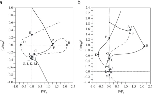
Fig. 5.Nonlinear equilibrium paths of theL-frame forSc¼5EI/L. (a) Rotationyand (b) displacementw.

-1.0

P/P_e -1.0

-0.8 -0.6 -0.4 -0.2 0.0 0.2 0.4 0.6 0.8 1.0

(

ω

/

ω0

)

2

(

ω

/

ω0

)

2

F

G, I, K, M H

L J E

D A _B

C

-0.4 -0.2 0.0 0.2 0.4 0.6 0.8 1.0 1.2 1.4 1.6 1.8 2.0 2.2 2.4

A

B

C D

E F

G

H I J L

M K

-0.5 0.0 0.5 1.0 1.5 2.0 2.5 -1.0

P/P_e

-0.5 0.0 0.5 1.0 1.5 2.0 2.5

(4)

paths, and calculate the vibration frequencies and modes along these paths. Therefore, one can identify the stable and unstable branches of these paths and study how the modes and frequencies vary as a function of static pre-loading. The Newmark method together with a variable time increment adaptive strategy is used in the nonlinear free and forced vibration analysis. The geometric nonlinear ﬁnite element formulation for frames with rigid

connections implemented here is based on work by Alves[42], Yang and Kuo[43], and Galvao~ [44]. The consideration of semi-rigid connections is based on the ﬁnite element formulation proposed by Chan and Chui[39].

2. The nonlinear static equilibrium and free vibration problems

In the ﬁnite element method context, the equilibrium of any structural system can be expressed as

FiðuÞ ¼

l

Fr ð1Þ

whereFiis the internal forces vector, function of the generalized

displacement vectoru,

l

is a load factor, andFris a ﬁxed reference

vector deﬁning the direction and distribution of the applied load. To obtain the nonlinear equilibrium path of a structure, an incremental technique for the response is used to solve the system of equations (1). This procedure basically consists of calculating a sequence of incremental displacements,

D

ui, that

correspond to a sequence of given load increments

D

li

. However, asFiis a nonlinear function of the displacements, the estimated

solution for the problem (predicted solution:

D

l

0,

D

u0) for each load step normally does not satisfy Eq. (1). Consequently, a residual force vectorgis deﬁned

g¼

l

FrFiðuÞ ð2Þ

If the unbalanced forces represented by gdo not satisfy the convergence criteria, a new estimate for the displacements is

L L θ

Sc

1.37 0 2 4 6 8 10 12

θ

(deg)

S_c= 5 EI/L Sc → ∞

1.419 Hz

Frequency (Hz)

1.38 1.39 1.40 1.41 1.42 1.43

Fig. 7.Nonlinear frequency–amplitude relation for selected values of the connection stiffnessSc.

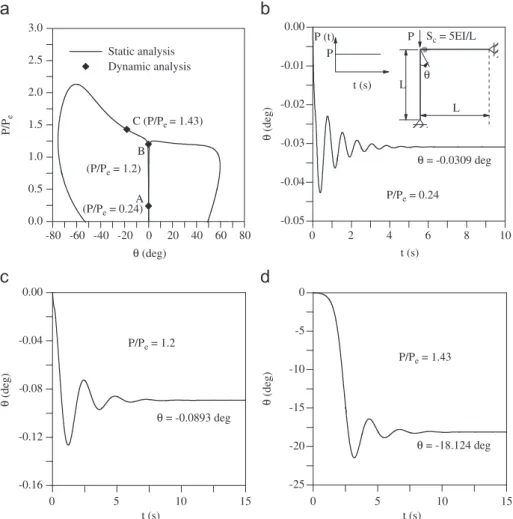
-80 0.0 0.5 1.0 1.5 2.0 2.5 3.0

Static analysis Dynamic analysis

A (P/Pe = 0.24) B

0 -0.05 -0.04 -0.03 -0.02 -0.01 0.00

θ

(deg)

L L θ

P Sc = 5EI/L P (t)

P

t (s)

0 -0.16 -0.12 -0.08 -0.04 0.00

θ

(deg)

-25 -20 -15 -10 -5 0

θ

(deg)

θ = -18.124 deg

P/P

e

θ (deg) t (s)

-60 -40 -20 0 20 40 60 80 2 4 6 8 10

t (s)

P/Pe = 1.43 P/Pe = 0.24

θ = -0.0309 deg C (P/Pe = 1.43)

(P/Pe = 1.2)

P/Pe = 1.2

θ = -0.0893 deg

5 10 15 0

t (s)

5 10 15

(5)

obtained by the relation

Kt

d

u¼g ð3Þ

whereKtis the tangent stiffness matrix of the structural system

and

d

uis the residual displacement vector.

The estimate of the correction

D

uis not directly obtained by solving Eq. (3). Instead, the residual displacement vector is deﬁned as a sum of two components[43,44]:

d

u¼

d

ugþ

dld

ur ð4Þ

where

dl

is a load parameter that, to make the correction process more efﬁcient, is evaluated in an iterative cycle that also corrects the load increment, and

d

ugand

d

urare obtained by

d

ug¼Kt1g ð5aÞ

d

ur¼Kt1Fr ð5bÞ

These displacement vectors can be easily obtained sinceKt,g, and Fr are known. The deﬁnition of

dl

in Eq. (4) depends on a

constraint equation to be added to the nonlinear problem (for example, an arc-length constraint equation).

The vibration frequencies and the corresponding modes of vibration in a loaded structure can be obtained by solving the following eigenvalue problem:

½ðKLþKtÞ

o

2MX¼0 ð6Þ

whereKLandKtare the linear and geometric stiffness matrices,

respectively,Mis the mass matrix, which also considers the effect of the semi-rigid connection,

o

is the natural frequency, andXis the vibration mode vector. Appendix A illustrates the step-by-step numerical procedures for solving the static nonlinear problem and, subsequently, calculating the natural frequencies and vibration modes.

2.1. Semi-rigid connections

In this work, the consideration of semi-rigid connections is based on the ﬁnite element formulation proposed by Chan and Chui [39], where the connection is represented as a rotational linear spring with stiffnessSc¼kEI/L. In the elastic global analysis L

L θ

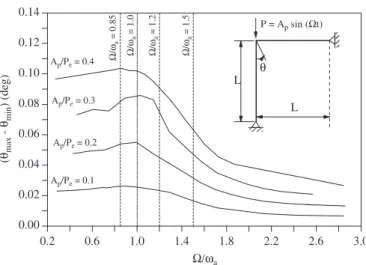
0.2 0.00 0.02 0.04 0.06 0.08 0.10 0.12 0.14

Ap/Pe = 0.1 Ap/Pe = 0.2 Ap/Pe = 0.3 Ap/Pe = 0.4 Ω

/

ωa

= 0.85

Ω

/

ωa

= 1.0

Ω

/

ωa

= 1.2

Ω

/

ωa

= 1.5

(

θmax

-

θmin

) (deg)

0.6 1.0 1.4 1.8 2.2 2.6 3.0

Ω/ω_a

P = A_p sin (Ωt)

Fig. 9.Resonance curves for theL-frame with rigid connections submitted to a harmonic load concentrated on the top of the column.

-0.04 -0.4 -0.2 0.0 0.2 0.4

θ

(deg/s)

θ

(deg/s)

θ

(deg/s)

θ

(deg/s)

-0.08 -0.6 -0.4 -0.2 0.0 0.2 0.4 0.6

-0.06 -0.6 -0.4 -0.2 0.0 0.2 0.4 0.6

-0.08 -0.4 -0.2 0.0 0.2 0.4 θ (deg)

-0.02 0.00 0.02 0.04 -0.04 0.00 0.04 0.08 θ (deg)

θ (deg) θ (deg)

-0.04 -0.02 0.00 0.02 0.04 -0.04 0.00 0.04 0.08

(6)

of frames the joints are usually classiﬁed in some design codes according to their rotational stiffnessScas nominally pinned, rigid

and semi-rigid. For example, according to Eurocode 3[50], the stiffness of the beam-to-column connections,Sc¼kbEIb/Lb, can be

classiﬁed as:

Nominally pinned, forkbr0.5.

Semi-rigid, for 0.5okbrk¯b.

Rigid, forkbZk¯b.

wherek¯b¼8 for braced frames where the bracing system reduces

the horizontal displacement by at least 80% andk¯b¼25 for other

frames provided that in every storey kb/kcZ0.1. Here the

subscriptbrefers to beam andcto column.

3. The nonlinear transient problem

In the ﬁnite element context, the nonlinear time response of the structure can be obtained by solving the following set of discrete equations of motion:

Mu€þCu_þFiðuÞ ¼

l

ðtÞFr ð7Þ

where M and C are the mass and viscous damping matrices, respectively, andFiis the internal force vector that depends on the

displacement vectoruof the system,u_andu€ are the velocity and acceleration vectors, respectively, and [

l

(t)Fr] is the external

excitation vector.

The solution of the nonlinear dynamic system (7) can be obtained through a time integration algorithm together with adaptive strategies for the automatic increment of the time step. The numerical methodology used here is presented in Appendix B.

The numerical integration algorithm is based on the work by Dokainish and Subbaraj[45], while the time increment strategy is based on work by Jacob[46]. Details of the nonlinear dynamic formulation as well as the computational program are found in Galvao~ [44].

3.1. Nonlinear vibration analysis

The nonlinear frequency–amplitude relation provides funda-mental information on the nonlinear vibration analysis of any structural system, and it gives a good indication of the type

L = 1000 mm z0 = 20 mm _{h = 20 mm}

h

w P (N/mm)

Sc Sc

E = 210000 MPa ρ = 78 x 10-9 Ns2 /mm4

P (t)

t (s) P (t)

P

t (s)

P (t) = Ap sin (Ωt)

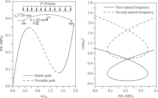
Fig. 12.Arch with semi-rigid joints under static and dynamic loading. w P (N/mm)

Sc Sc

z0 = 20

mm h = 20 mm h

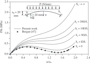
0.0 0.0 0.5 1.0 1.5 2.0 2.5

P/h (MPa)

Present work Bergan [47]

S_c = 0 S_c = EI/L S_c = 5EI/L S_c = 10EI/L S_c = 20EI/L

Sc → ∞

w/z0

0.4 0.8 1.2 1.6 2.0 2.4

Fig. 13.Arch nonlinear equilibrium paths for different joint stiffness valuesSc.

0.0 -40

0 40 80 120

ω

2 (x10 -3) (rad/s)

2

A2 B2 A1 B1_C 2 C1

(A1) P/h = 0.3454

(A2) P/h = 0.0789

(B1) P/h = 0.3916

(B2) P/h = 0.1944

(C1) P/h = 0.5212

(C2) P/h = 0.4737 Sc = 0

Sc = EI/L

Sc = 5EI/L

Sc = 10EI/L

Sc = 20EI/L Sc→ ∞

P/h (MPa)

0.2 0.4 0.6 0.8 1.0 1.2

Fig. 14.Inﬂuence of the static pre-load on the lowest natural frequency of a shallow arch for different joint stiffness valuesSc.

0.2 2 4 6 8 10 12 14

ApL/Pe = 0.1

ApL/Pe = 0.15

ApL/Pe = 0.2

ApL/Pe = 0.3

ApL/Pe = 0.4

L L

θ

q (t) = Ap sin(Ωt) kN/cm

(θmax

-

θmin

) (deg)

Ω/ωa

0.4 0.6 0.8 1.0 1.2 1.4

ApL/Pe = 0.5

(7)

(hardening or softening) and degree of nonlinearity of the system. Various approaches, including perturbation methods and the harmonic balance method, have been developed to study non-linear oscillators with a small number of degrees of freedom. Here the methodology proposed by Nandakumar and Chatterjee[48]is used to obtain this relation using the ﬁnite element method. First, the nonlinear equations of motion are numerically integrated, and the time response of the slightly damped system is obtained for a chosen node. Then, the maximum amplitude and corresponding period between two consecutive positive peaks are computed at each cycle. Consider two successive peaks at times T1 and T2. Let their average value beA1and let the trough between these

two positive peaks be A2. We then deﬁne the amplitude as

A¼(A1A2)/2 and the frequency as f¼1/(T1T2). The resulting amplitude and frequency values are plotted to give the frequency–amplitude relation. To obtain the peak amplitudes with the necessary accuracy, a small time step must be imposed

in the integration process. In addition, a large number of elements are necessary to describe accurately the large amplitude response of the structure.

Low-dimensional numerical models employ relatively easy techniques for obtaining nonlinear resonance curves. In contrast, it is extremely computationally difﬁcult to obtain these curves for structural systems with a large number of degrees of freedom. Here, a simple repetitive procedure coupled with the integration method is implemented, which consists of giving constant excitation–frequency increments

D

O

and, for each incremental step, integrating the differential equations of motion during N

harmonic excitation cycles. The response of the initial cycles associated with the short transient response is dismissed, and the maximum amplitude of the steady-state solution is plotted as a function of the forcing frequency. Of course, this brute force method is unable to obtain unstable branches of resonance curves. In the developed program, theNand

D

O

parameters are

h = 20 mm h

w

z0 = 20 mm

P (N/mm)

0.0

w/z0

0.0 0.1 0.2 0.3 0.4 0.5

P/h (MPa)

Stable path Unstable path

0.0 -0.4

0.0 0.4 0.8 1.2 1.6 2.0 2.4 2.8

(

ω

/

ω0

)

2

First natural frequency Second natural frequency

P/h (MPa)

0.4 0.8 1.2 1.6 2.0 0.1 0.2 0.3 0.4

Fig. 15.Arch equilibrium paths and natural frequency–load relation forz0¼20 mm.

h = 20 mm h

w P (N/mm)

0.0 -0.5

0.0 0.5 1.0 1.5

P/h (MPa)

-0.5 -1.0 -0.5 0.0 0.5 1.0 1.5 2.0

w/z₀

0.4 0.8 1.2 1.6 2.0 0.0 0.5 1.0 1.5

P/h (MPa)

(

ω

/

ω0

)

2

z0 = 30 mm

(8)

deﬁned by the user, together with the integration method to be used, and then an adaptive strategy for the variable time incre-ment is applied[46].

4. Numerical examples

Three structural problems are used to test the formulation and to show the possible buckling and vibration characteristics of slender frames: an L-frame, a shallow arch, and a pitched-roof frame. The free vibration analyses involve the calculation of the natural frequencies and vibration modes and the load–frequency relation. This study is fundamental for understanding the process of stability loss in structures with a high degree of nonlinearity and complicated equilibrium paths. Their nonlinear behavior under dynamic loads is also veriﬁed.

4.1. L-frame

In Galvao et al.~ [24], a detailed parametric analysis of the elastic stability ofL-frames was performed. The geometrical and physical properties of the frame are presented inFig. 1.

4.1.1. Instability and vibration analysis

L-frames usually display an asymmetric bifurcation, character-ized by an initial non-zero slope of the post-critical equilibrium path. Galvao et al.~ [24]observed that, when the stiffness of the beam–column connection increases, the frame’s critical load increases, and the initial slope of the asymmetric post-critical path simultaneously increases, resulting in the structure becom-ing more sensitive to initial imperfections. This characteristic is

shown inFig. 2, where the variation of the load parameterP/Peis

plotted as a function of the node rotation,

y

, for different values of the connection stiffness parameterSc. Pe is the Euler critical

load. Small perturbations are used in the numerical strategy to obtain the two branches of the post-critical path. AsSc-0, the

inﬂuence of the lateral bracing decreases, and the post-buckling path approaches that of a simply supported column (pinned connection).

The nonlinear relation between the load parameter and the natural frequencies for different values of joint stiffness is given inFig. 3. This relation not only shows the inﬂuence of the static

0.0 -1.6 -1.2 -0.8 -0.4 0.0 0.4 0.8 1.2 1.6 2.0 2.4 2.8 3.2

P/h (MPa)

h = 20 mm

h

w

z0 = 40 mm

P (N/mm)

-2.0 -2.5 -2.0 -1.5 -1.0 -0.5 0.0 0.5 1.0 1.5 2.0 2.5 3.0

(

ω

/

ω0

)

2

w/z0 P/h (MPa)

0.4 0.8 1.2 1.6 2.0 -1.5 -1.0 -0.5 0.0 0.5 1.0 1.5 2.0 2.5

Fig. 17. Arch equilibrium paths and natural frequency–load relation forz0¼40 mm.

z0 = 20 mm

ω = 372.82 rad/s

ω = 246.21 rad/s

z0 = 30 mm

ω = 353.46 rad/s ω = 371.35 rad/s

z0 = 40 mm

ω = 369.32 rad/s

ω = 462.59 rad/s

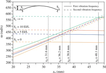
Fig. 18. Arch vibration modes for differentz0values. 20

200 250 300 350 400 450 500 550 600 650 700

ω

(rad/s)

z0

≅

31.6 mm

Sc = 5 EI/L

Sc = 0 Sc = 10 EI/L Sc → ∞

z0

≅

38.8 mm

z0

≅

48.1 mm

z0

≅

36.2 mm

First vibration frequency Second vibration frequency z0 Sc

z0 (mm)

25 30 35 40 45 50

Sc

(9)

pre-loading on the natural frequencies, but it can also be used, according to the dynamic stability criterion, to identify stable and unstable branches along the equilibrium paths: if

o

2₄_{0, the}

response is stable, while if

o

2

o0, the response is unstable.

Critical conditions are obtained for

o

2_¼₀_[49]_{. This relation has}

also been proposed as a tool for the experimental identiﬁcation of critical loads through a non-destructive vibration test using small static pre-loads[6].

Table 1 shows the variation of the ﬁrst three natural frequencies of the unloaded structure withSc. For highScvalues,

the natural frequencies are well spaced, but whenSc-0, the joint

approaches a perfect hinge, and the first two natural frequencies converge to the same value. Among the analyzed frequencies, the second frequency is influenced more by the connection stiffness than the other two. This can be explained by analyzing the three first vibration modes for Sc¼0 (pinned connection), Sc¼5EI/L

(semi-rigid connection), andSc-N(rigid connections) illustrated

inFig. 4. The variation of the angle between the bars withScis

larger for the second mode, leading to a larger contribution of the spring to the total stiffness of the system.

The static and dynamic post-critical behavior of the loaded

L-frame, with beam–column stiffness connection Sc¼5EI/L, is

illustrated in Figs. 5 and 6. Fig. 5a shows the variation of P/Pe

with

y

, while Fig. 5b shows the variation of the load with the vertical displacement of the node,w.Fig. 6shows the variation of the two first natural frequencies with the load up to very large displacements and rotations. Capital letters are used in these figures to identify some reference configurations in both figures. Continuous and dashed curves identify stable and unstable configurations, respectively. The results show that the static pre-load has a strong influence on both frequencies. Knowing that, in the regions of the trajectory where the equilibrium is stable, all the natural frequencies have real values, and that the corresponding regions with negative values of

o

2 _{are unstable}

(natural frequency with imaginary value), the stable and unstable equilibrium conﬁgurations can be deﬁned, as illustrated in Figs. 5

20 0 5 10 15 20 25 30 35 40 45

w (mm)

39.2 Hz

0.0 -40 -20 0 20 40 60 80

w (mm)

w

z0 = 20 mm

Frequency (Hz) Time (s)

25 30 35 40 45 0.2 0.4 0.6 0.8 1.0

Fig. 20.Frequency–amplitude relation and large amplitude nonlinear time response.

w h = 20 mm h

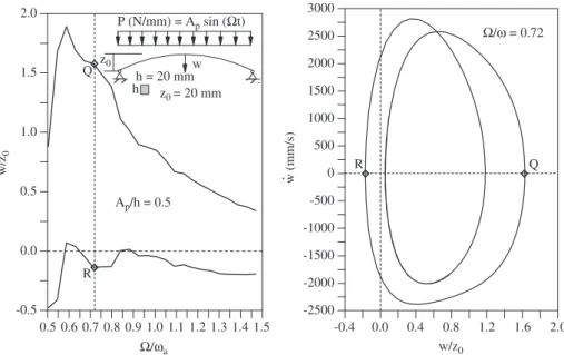
z0

z₀= 20 mm

0.5 -0.5

0.0 0.5 1.0 1.5 2.0

w/z

0

Ap/h = 0.5

Q

R

-0.4 -2500 -2000 -1500 -1000 -500 0 500 1000 1500 2000 2500 3000

w (mm/s)

Q R

Ω/ωa

0.6 0.7 0.8 0.9 1.0 1.1 1.2 1.3 1.4 1.5

w/z0

0.0 0.4 0.8 1.2 1.6 2.0

P (N/mm) = Ap sin (Ωt)

Ω/ω = 0.72

(10)

and 6. Through this analysis, various saddle-node bifurcations (fold points) are identiﬁed along the post-buckling path. The simultaneous calculation of the nonlinear path and the lowest natural frequencies associated with each equilibrium position has been shown to be a computationally easy and efﬁcient method for the analysis of the stability of the equilibrium paths.

4.1.2. Transient and resonance analysis

Fig. 7shows the frequency–amplitude relation obtained by the methodology described in Section 3.1 for different values ofScup

to very large deﬂections. For Sc¼0, the frame shows a slight

softening behavior; for higher values ofSc, the response becomes

of the hardening type, showing an increase of the nonlinear frequency with the vibration amplitude. Consider now the same

L-frame given inFig. 1with a beam–column stiffness connection

Sc¼5EI/Land a viscous damping matrix proportional to the mass

and stiffness matrices, C¼

a

M+

b

Kt, deﬁned by Rayleigh

coefﬁ-cients

a

and

b

, which are calculated here based on the critical damping coefﬁcient

x

¼0.12 of the ﬁrst and second modes. The frame behavior under a suddenly applied step load of inﬁnite

duration (Fig. 1a) is analyzed.Fig. 8shows the transientL-frame response under increasing load levels. The frame exhibits large amplitude vibrations during the transient phase and converges to the static conﬁguration corresponding to the applied load level.

For a harmonic load (Fig. 1b) and using the procedure described in Section 3.1, the resonance curves for theL-frame are obtained considering a perfectly rigid connection between the beam and the column for increasing values of the excitation amplitude,Ap.Fig. 9exhibits the variation of the amplitude of the

steady state solution9

ymax

ymin

9with the frequency ratio

O

/

o

a,

where

O

is the excitation frequency of the harmonic load and

o

a¼

o

0

ffiffiffiffiffiffiffiffiffiffiffiffi

1

x

2 q

is the ﬁrst natural frequency of the damped frame. The inﬂuence of the nonlinearity is small, which is explained by the frequency–amplitude relation shown inFig. 7. However, asApincreases, the resonance peak moves to a higher

frequency range due to the hardening character of the nonlinearity. The phase planes of the steady-state response for

Ap/Pe¼0.4 and selected values for the excitation frequency are

presented inFig. 10. The asymmetry of the response with respect to

y

(9

ymax

9o9

ymin

9) is due to the asymmetric character of the frame nonlinearity, leading to the presence of both quadratic and cubic nonlinearities in the equations of motion.

A similar analysis is performed here considering a distributed harmonic load along the beam. The resonance curves are depicted inFig. 11. In this case, contrary to the previous one, a marked softening behavior is observed, with the resonant peak moving to the lower frequency range. As shown by Galvao et al.~ [24], the nonlinear equilibrium path of this frame exhibits a strong nonlinearity associated with a signiﬁcant loss of initial stiffness. The same inﬂuence of this type of load is now observed on the dynamic nonlinear response.

4.2. Shallow arch

The dynamic response of shallow arches has been extensively analyzed due to their practical applications in the various branches of engineering, particularly in large civil engineering structures. Consider an arch with semi-rigid supports submitted to a uniformly distributed vertical loadP, as illustrated inFig. 12.

0.5 -0.5

0.0 0.5 1.0 1.5 2.0

w/z

0

A_p/h = 0.5 Ap/h = 0.4

A_p/h = 0.3 A_p/h = 0.2

w h = 20 mm h z0

Ω/ωa

0.6 0.7 0.8 0.9 1.0 1.1 1.2 1.3 1.4

P (N/mm) = Ap sin(Ωt)

z0 = 20 mm

Fig. 22.Arch resonance curves for different amplitudes of the harmonic excitation.

w h = 20 mm h z0

z0 = 20 mm

0.4 -0.4

0.0 0.4 0.8 1.2 1.6 2.0

w/z

0

Ap/h = 0.5

132.9 -0.4

0.0 0.4 0.8 1.2 1.6 2.0

w/z

0

Ω/ωa t (s)

0.6 0.8 1.0 1.2 1.4 1.6 133 133.1 133.2 133.3 133.4 Ω/ωa = 0.72

P (N/mm) = A_p sin (Ωt)

(11)

Fig. 13 shows the nonlinear equilibrium paths for increasing values of the connection stiffnessSc. For a simply supported arch

(Sc¼0) the present results agree well with those obtained by Bergan [47]. For small values of Sc, two limit points (fold bifurcations)

separating the intermediate unstable path from the two stable branches are observed. AsScincreases, the limit points disappear

and the arches exhibit highly nonlinear ascending equilibrium paths. The nonlinear relation between the load and the lowest natural frequency for different values of the connection stiffness is given in

Fig. 14. As shown above, this relation not only shows the inﬂuence of static pre-loading on the natural frequencies, but can also be used to identify stable and unstable branches along the equilibrium paths according to dynamic stability criteria. In the present analysis, the unstable branches are located between the two limit points of the equilibrium paths (A1, A2, B1, B2, C1, and C2). The literature describes

various types of arches, particularly shallow-arches designed for roofs that have lost their stability due to the deterioration of the supports. Corrosion is one of the most frequent causes for the loss of stiffness of the support. In this case, there is a slowly decreasing value for Sc and, consequently, a marked decrease in the overall

structure stiffness and dynamic characteristics, as shown herein. These changes can only be evaluated through detailed analysis of the nonlinear structural behavior.

AsScor the arch height increases, before the load reaches the

upper limit point value, the arch may lose stability through an unstable bifurcation, upon which the arch assumes an asym-metric conﬁguration. Figs. 15–17 show the nonlinear equilibrium

path of a sinusoidal pinned arch for three values with a heightz0

(20, 30, and 40 mm, respectively) and the variation of the two lowest natural frequencies as a function of the static pre-load.

Fig. 18exhibits the ﬁrst two vibration modes for the three differ-ent values ofz0. For small values ofz0, the ﬁrst mode is always symmetric, and the second asymmetric, and the two frequencies are well spaced. As the z0 increases, the frequencies approach each other, and for a critical value ofz0, the frequency associated with the asymmetric frequency mode becomes lower than that of the symmetric mode. This occurs at the point when the structural instability transitions from limit point to unstable bifurcation, since the same nonlinearity that changes the loss of stability mechanism also changes the modal form.

The variation of the ﬁrst two natural frequencies of the arch as a function ofz0is illustrated inFig. 19for different values of the semi-rigid connection Sc. While the frequency associated with

the symmetric mode increases linearly with z0, the frequency associated with the asymmetric mode remains nearly constant. For Sc¼0 and z0ﬃ31.6 mm, the ﬁrst two frequencies are

practically coincident. The value ofz0where this crossing occurs increases with Sc. In structures with accentuated nonlinear

behavior, this often occurs and creates various internal resonance phenomena.

4.2.2. Transient and resonance analysis

Fig. 20 shows a typical frequency–amplitude relation for a shallow arch showing the initial softening behavior and the

-0.002 0.00 0.02 0.04 0.06 0.08 0.10 0.12 0.14

P/P

e

Sc = 0 Sc = EI/L Sc = 5EI/L Sc = 1015EI/L

P

P P P

P

Sc Sc

w

0.00 -0.2

0.0 0.2 0.4 0.6 0.8 1.0

(ω

/

ω0

)

2

Sc = 0 _S c = EI/L

Sc = 1015EI/L

w/L P/Pe

0.02 0.04 0.06 0.08 0.10 0.12 0.14 0.000 0.002 0.004 0.006 0.008 0.010

Sc = 5EI/L

Fig. 25. Inﬂuence of the semi-rigid joint stiffnessScon the nonlinear equilibrium paths and frequency–load relation. P

P

P P P

P

14 m 14 m

L = 5 m h = 1.471 m

E = 2.1x108 kN/m2 A = 0.007273 m2 I = 0.0001627 m4 ρ = 7.8 kNs2/m4

Sc Sc

(12)

change from softening to hardening at large deflections, due to increasing flexural stiffness. A typical nonlinear time response starting at a highly deformed configuration in the form of the first vibration mode is also shown in Fig. 20, where the nonlinear variation of amplitude with the vibration period is clearly shown. The dynamic response of the arch under a uniformly distributed harmonic is investigated next. A pinned arch with

z0¼20 mm is considered. Fig. 21 shows the variation of the maximum and minimum amplitude of the response as a function of the forcing frequency parameter

O

/

o

a for an excitation

amplitude relationAp/h¼0.5 MPa.

o

a¼238.4 rad/s is the lowest

natural frequency. Fig. 21 also displays a phase diagram for

O

/

o

a¼0.72.

Fig. 22 illustrates the non-dimensional vertical displacement of the arch mid-spanw/z0as a function of

O

/

o

afor various values

ofAp/h. When the excitation magnitude increases, the resonance

peaks move sharply to the lower frequency range, indicating a strong softening behavior in agreement with the frequency– amplitude relation shown in Fig. 20. This behavior is also

compatible with the type of nonlinearity observed in the system’s static solution. As is typical of nonlinear systems, the resonance curve begins to bend atAp/h¼0.4 in a region of low

frequencies, which produces more than one permanent solution for the same frequency value. When the magnitude of excitation reaches Ap/h¼0.5, the amplitude increases considerably in the

low frequency region up to the point where the arch loses stability and inverts its concavity. Before this phenomenon occurs, period multiplying bifurcations are observed. A typical solution for this region is shown in Fig. 23a, and its time response is presented in Fig. 23b. The points highlighted in Fig. 23 correspond to the points of the Poincare´ section of the steady-state solutions, which clearly indicate the duplication of the period.

4.3. Pitched-roof frame

The numerical strategy developed is now applied to the analysis of a pitched-roof frame with beam–column ﬂexible

-0.004 0.00 0.02 0.04 0.06 0.08 0.10 0.12 0.14 0.16

w/L

h = 0

h = 1.471 m

h = 0.5 m

h = 1.0 m

-0.002 0.00 0.02 0.04 0.06 0.08 0.10 0.12 0.14 0.16 0.18 0.20 0.22

w/L

h = 2.0 m

h = 1.471 m h = 5.0 m

h = 3.0 m h = 4.0 m

P

P P P

P w

L+h

P/Pe P/Pe

-0.002 0.000 0.002 0.004 0.000 0.002 0.004 0.006 0.008 0.010

Fig. 27.Variation of the nonlinear equilibrium path with the parameterh. Symetric mode

Asymetric mode

ω01

ω02

0.00 -0.5

0.0 0.5 1.0 1.5 2.0

(

ω

/

ω0

)

2

A

A E

E D

D B

B C

C

F F

-0.002 0.00 0.02 0.04 0.06 0.08 0.10 0.12 0.14 0.16

w/L

Stable path Unstable path A

D

E B

C

F

P/P_e P/P_e

0.02 0.04 0.06 0.08 0.10 0.12 0.14 0.000 0.002 0.004 0.006 0.008 0.010

(13)

joints, as shown in Fig. 24. Twenty ﬁnite elements are used here to model the structure.

Fig. 25a shows the nonlinear equilibrium paths for increasing values of the joint stiffness Sc. The nonlinear relation between

the load and the natural frequencies for different values of joint stiffness is given in Fig. 25b. The applied load is non-dimensionalized by Pe¼

p

2EI/L2, and the frequencies are

non-dimensionalized by the lowest free vibration frequency of the unloaded frame with rigid connections,

o

0¼23.912 rad/s. For the frame with rigid connections, the lowest natural frequency is associated with a symmetric ﬂexural vibration mode, while the second lowest frequency is associated with an asymmetric ﬂexural mode, as shown in Fig. 26, which presents the variation of these two frequencies along the pre- and post-buckling path.

Fig. 27 illustrates the variation of the nonlinear equilibrium path with the geometric parameterhof the pitched-roof frame

Vibration mode associated with ω01

0.00 -200

0 200 400 600 800 1000 1200

ω

2 (rad/s)

2

ω01

ω02

0.00 -200

0 200 400 600 800 1000 1200

ω

2 (rad/s)

2 _ω

01

ω02

0.00 -300

0 300 600 900 1200

ω

2 (rad/s)

2

ω01

ω02 Vibration mode

associated with ω02

0.00 -500 -250 0 250 500 750 1000 1250

ω

2 (rad/s)

2

ω01

ω02

P/Pe P/Pe

0.02 0.04 0.06 0.08 0.10 0.02 0.04 0.06 0.08 0.10 0.12 0.14

0.03 0.06 0.09 0.12 0.15 0.18 0.04 0.08 0.12 0.16 0.20

Fig. 28.Variation of the ﬁrst two natural frequencies (o01ando02) and their corresponding vibration modes with the parameterh. (a)h¼0, (b)h¼1.471 m, (c)h¼3 m and (d)h¼4 m.

1.2 0.0 0.4 0.8 1.2 1.6 2.0 2.4 2.8

Sc = 0 Sc = EI/L Sc → ∞

3.81 Hz

1.71 Hz 2.83 Hz

v

Sc Sc

v (m)

Frequency (Hz)

1.6 2.0 2.4 2.8 3.2 3.6 4.0

(14)

(see Fig. 24) and Fig. 28 shows the variation of the two lowest natural frequencies of the frame with the applied load P for selected values ofhtogether with the corresponding free vibration modes. For small values ofh,the two lowest frequencies are well separated for any load value. The lowest frequency corresponds to a symmetric ﬂexural mode, while the second frequency corresponds to an asymmetric mode. As the height of the roof increases, the curves corresponding to these modes approach each other and ﬁnally intersect, at a certain value ofP/Pe(see the results

forh¼3 m), and, after this point, the lowest frequency becomes associated with the asymmetric mode. Ifhincreases still further, the difference between the frequencies increases again, as shown in the ﬁgure forh¼4 m. Again the variation of these frequencies shows that these frames may display various types of internal resonance and exhibit a complex dynamic.

Finally, Fig. 29 shows the frequency–amplitude relation of the pitched-roof for three selected values of the stiffness of the semi-rigid connection. The relation is almost linear for small-to-medium amplitude oscillations of the softening type when very large vibration amplitudes occur, which is outside the range of practical applications.

Although this paper is restricted to the elastic nonlinear behavior of slender frames, one must have in mind that buckling may occur in the elastic range but added stresses due to bending may cause the combined stress to exceed the elastic stress range, or either due to several factors such as residual stresses, initial geometric imperfections and inherent nonlinearity of the stress– strain relationship, the buckling loads may occur in the inelastic range. This occurs in most civil engineering applications and, in such cases, the stability and vibration analysis must be conducted taking into account large deﬂections and plastiﬁcation of members and joints with the consequent force redistributions. In this case, the nonlinear dynamic analysis must include the cyclic behavior of the semi-rigid joints[51].

5. Conclusions

The results presented in this paper indicate that the precise evaluation of the connection stiffness, a key point in the design of metal structures, is essential for the calculation of critical conditions. This is particularly important for practical application where damage usually occurs at the connections, decreasing their stiffness and radically changing the nonlinear behavior of the frame.

The results also indicate that the loss of stiffness of a connection during the service life of the structure may signiﬁ-cantly affect the structural behavior under both static and dynamic loads. This is in agreement with the literature describing structural failures due to support deterioration. In these cases, there is a slow decrease in the joint stiffness Sc value with

accentuated changes in the overall stiffness of the structure and in its dynamic characteristics, which can only be detected and quantified by detailed nonlinear behavior analyses of the structure. The results also show the influence of semi-rigid connections and static pre-loading on the natural frequencies of the analyzed frames. To obtain a better understanding of the instability phenomena of these structures, the nonlinear fre-quency–amplitude relation is numerically obtained, and the forced vibrations of these structures when submitted to different dynamic loads are analyzed. The methodology used to obtain the resonance curves and frequency–amplitude relation involves the use of computer-intensive and time-consuming procedures. One approach to solve this problem is the use of precise reduced order models or the implementation of efficient continuation techni-ques for dynamic bifurcation analysis together with the FE method.

Acknowledgments

The authors wish express their gratitude to CAPES and CNPq for the support received in the development of this research. They also thank FAPEMIG and FAPERJ (Minas Gerais and Rio de Janeiro State Foundations) for the ﬁnancial support. Special thanks go to Harriet Reis for her editorial reviews.

Appendix A

SeeTable A1.

Table A1

Algorithm for nonlinear static solution and vibration analysis.

1. Input the material and geometric properties of the frame 2. Obtain the reference force vectorFr

3. Displacements and load parameter in the actual equilibrium conﬁguration: t_u_,t_l

4.INCREMENTAL TANGENT SOLUTION:Dl0_and_Du0 4.1. Calculate the tangent stiffness matrixKt 4.2. Solve:dur¼K1

t Fr

4.3. DeﬁneDl0_{with a determined strategy for the load increment:}

Dl0_¼₇_D_l =

ffiffiffiffiffiffiffiffiffiffiffiffiffiffiffiffiffiffiffiffiffiffiffiffiffiffiffiffiffiffiffi duT

rdurþFTrFr q

,Dl: arch-length, Crisﬁeld [26] or,

Dl0¼71Dl0

ffiffiffiffiffiffiffiffiffiffiffiffiffiffiffiffiffiffiffiffiffiffiffiffiffiffiffiffiffiffiffiffiffiffiffiffiffiffiffiffiffiffiffiffiffiffiffiffiffiffiffiffiffiffiffiffi 1

duT r 1

dur

= tduT rdur

r

, Yang and Kuo[43]

4.4. Calculate:Du0_¼Dl0_d_ur

4.5. Update the variables in the new equilibrium conﬁgurationt+Dt tþDt

l¼tlþDl0andtþDt_u_¼t_u_þ_Du0

5.NEWTON–RAPHSON ITERATION FORk¼1, 2,y,Ni

5.1. Calculate the internal forces vector of the current conﬁguration: tþDt_Fðk1Þ

i ¼tFþKtDuðk1Þ

5.2. Calculate the unbalanced forces vector:

gðk1Þ_¼tþDt

lðk1Þ_F

rtþDtFðik1Þ

5.3. Verify the convergence:99g(k1)₉₉_/₉₉_D_l(k1)_F

r99rx, withxbeing the tolerance factor

YES: stop the iteration cycle and go to item 5.8

5.4. Obtaindlk_{using an iteration strategy:}

dlk¼ ðDu0_ÞT_d_uk_g=_ðð_Du0_ÞT_þ_D_l0_FT rFrÞ, or, dlk¼ tduT

rdukg= t

duT rdukr

, Galvao~ [44]

5.5. Determine:duk_¼_d_uk

gþdlkdukr, with:

duk

g¼ Kt1ðk1Þgðk1Þanddukr¼Kt1ðk1ÞFr

5.6. Update the load parameters and the displacement vectors: (a) Incrementals:Dlk_¼_D_l(k1)₊_dlk_and_Duk_¼_Du(k1)₊_d_uk (b) _Totals:tþDt

l¼tlþDlkandtþDt_uk_¼t_u_þ_Duk

5.7. Return to Step 5

5.8. Determine the natural frequencies and the associated vibrations modes:

(a) Update the tangent stiffness matrixK¼KL+ Ktand the mass matrixM

(b) Decompose theMmatrix by the Cholesky Method:M¼ST_S (c) Calculate:Q¼S1_{and determine:}_A_¼_QT_KQ

(d) Solve the eigenvalue problemAX¼lXby using the Jacob Method

[44]obtaining the eigenvalues (o2_{) in the diagonal of matrix}_A and the eigenvectors (vibration modes) in the columns of matrixX.

(15)

Appendix B

SeeTable B1.

References

[1] Simitses GJ. Effect of static preloading on the dynamic stability of structures. AIAA Journal 1983;21(8):1174–80.

[2] Simitses GJ. Dynamic stability of suddenly loaded structures. Springer; 1990. [3] Wu TX, Thompson DJ. The effects of local preload on the foundation stiffness and vertical vibration of railway track. Journal of Sound and Vibration 1999;219(5):881–904.

[4] Machado SP, Cortı´nez VH. Free vibration of thin-walled composite beams with static initial stresses and deformations. Engineering Structures 2007;29:372–82.

[5] Zeinoddini M, Harding JE, Parke GAR. Dynamic behaviour of axially pre-loaded tubular steel members of offshore structures subjected to impact damage. Ocean Engineering 1999;26(10):963–78.

[6] Gonc-alves PB. Axisymmetric vibrations of imperfect shallow spherical caps

under pressure loading. Journal of Sound and Vibration 1994;174(2):249–60. [7] Massonnet Ch. An accurate approximate formula for assessing the vibration frequency of structures axially loaded. International Journal of Mechanical Sciences 1972;14(11):729–34.

[8] Williams FW. Simple buckling and vibration analyses of beam or spring connected structures. Journal of Sound and Vibration 1979;62(4):481–91. [9] Rosman R. Buckling and vibrations of spatial building structures. Engineering

Structures 1981;3(4):194–202.

[10] Leissa AW, Kang J-H. Exact solutions for vibration and buckling of an SS–C– SS–C rectangular plate loaded by linearly varying in-plane stresses. Interna-tional Journal of Mechanical Sciences 2002;44(9):1925–45.

[11] Ganesan N, Kadoli R. Buckling and dynamic analysis of piezothermoelastic composite cylindrical shell. Composite Structures 2003;59(1):45–60. [12] Nieh KY, Huang CS, Tseng YP. An analytical solution for in-plane free

vibration and stability of loaded elliptic arches. Computers & Structures 81(13):1311–27.

[13] Xu R, Wu Y-F. Free vibration and buckling of composite beams with interlayer slip by two-dimensional theory. Journal of Sound and Vibration 2008; 313(3–5):875–90.

[14] Souza MA. The inﬂuence of changing support conditions on the vibration of buckled plates. Thin-Walled Structures 1994;18(2):133–43.

[15] Tada M, Suito A. Static and dynamic post-buckling behavior of truss structures. Engineering Structures 1998;20(4–6):384–9.

[16] Lestari W, Hanagud S. Nonlinear vibration of buckled beams: some exact solutions. International Journal of Solids and Structures 2001;38(26–27): 4741–57.

[17] Boutyour EH, Azrar L, Potier-Ferry M. Vibration of buckled elastic structures with large rotations by an asymptotic numerical method. Computers & Structures 2006;84(3-4):93–101.

[18] Soong TT, Dargush GF. Passive energy dissipation systems in structural engineering. Chichester: John Wiley & Sons; 1997.

[19] Galambos TV. Guide to stability design criteria for metal structures. 5th ed. Wiley; 1998.

[20] Koiter WT. Post-buckling analysis of simple two-bar frame. In: Broberg B, Hult J, Niordson F, editors. Recent progresses in applied mechanics; 1967. p. 337–54.

[21] Roorda J. The instability of imperfect elastic structures, PhD thesis, University College London, England, 1965.

[22] Silvestre N, Camotim D. Coupled global instabilities in pitched-roof frames. In: Camotim D, Dubina D, Rondal J, editors. Proceedings of the third international conference on coupled instabilities in metal structures: CIMS; 2000. p. 475–87.

[23] Silvestre N, Camotim D. Elastic buckling and second-order behaviour of pitched-roof steel frames. Journal of Constructional Steel Research 2007;63(6):804–18.

[24] Galvao AS, Gonc~ -alves PB, Silveira RAM. Post-buckling behavior and

imperfection sensitivity of L-frames. International Journal of Structural Stability and Dynamics 2005;5:19–38.

[25] Lee SL, Manuel FS, Rossow EC. Large deflection analysis and stability of elastic frames. Journal of Engineering Mechanics Divison ASCE 1968;94:521–47. [26] Crisfield MA. Nonlinear finite element analysis of solids and structures. John

Wiley & Sons; 1991.

[27] Blevins RD. Formulas for natural frequencies and mode shapes. Van Nostrand Reinhold; 1979.

[28] Chen WF, Goto Y, Liew JYR. Stability design of semi rigid frames. John Wiley & Sons; 1996.

[29] Barsan GM, Chiorean CG, Hu K. Computer program for large deﬂection elasto-plastic analysis of semi-rigid steel frameworks. Computers & Structures 1999;72:699–711.

[30] Kounadis AN, Ecomonou AP. The effects of the joint stiffness and of the constraints on the type of instability of a frame under follower force. Acta Mechanica 1980;36:157–68.

[31] Faella C, Piluso V, Rizzano G. Structural steel semirigid connections. theory, design and software. Boca Raton, FL: CRC Press LLC; 2000.

[32] Kawashima S, Fujimoto T. Vibration analysis of frames with semi-rigid connections. Computers & Structures 1984;19(1–2):85–92.

[33] Chan SL. Vibration and modal analysis of steel frames with semi-rigid connections. Engineering Structures 1994;16(1):25–31.

[34] Sophianopoulos DS. The effect of joint ﬂexibility on the free elastic vibration characteristics of steel plane frames. Journal of Constructional Steel Research 2003;59(8):995–1008.

[35] Shi G, Atluri SN. Static and dynamic analysis of space frames with nonlinear ﬂexible connections. International Journal for Numerical Methods in Engineering 1989;28:2635–50.

[36] Chan SL, Ho GWM. Nonlinear vibration analysis of steel frames with semirigid connections. Journal of Structural Engineering ASCE 1994;120(4): 1075–87.

[37] Chui PPT, Chan SL. Transient response of moment-resistant steel frames with ﬂexible and hysteretic joints frames. Journal Construction Steel Research 1996;39(3):221–43.

[38] Chui PPT, Chan SL. Vibration and deﬂection characteristics of semi-rigid jointed frames. Engineering Structures 1997;19(12):1001–10.

Table B1

Algorithm for nonlinear dynamic solution.

1. Input the material and geometric properties of the frame 2. Start the initial displacement, velocity and acceleration

vectorso_u

,

o_u_{_}_ando_u_€ 3. Form the mass matrixM 4.FOR EACH TIME STEPDt

4.1. Form the tangent stiffness matrixKtand the damping matrixC 4.2. Using Newmark parametersbandg, calculate the constants

a0¼ 1

bDt2,a1¼

g

bDt,a2¼

1 bDt,a3¼

1 2bDt1

,a4¼

g

b1,

a5¼ Dt

2 g

b2

,a6¼a0,a7¼ a2,a8¼ a3,

a9¼Dtð1gÞanda10¼gDt

4.3. Form the effective stiffness matrix:K^¼Ktþa0Mþa1C 4.4. Form the effective load vector:

^

F¼tþDtlFrþMa2tu_þa3tu€ þCa4tu_þa5tu€ tFi

4.5. Solve for displacement increments:KDu^ ¼F^

4.6. ITERATE CYCLE FOR DYNAMIC EQUILIBRIUM:k¼1, 2,y i. Evaluate the approximation of the acceleration, velocities

and displacements:

tþDt_u_€k_¼_a

0Duka2tu_a3tu€

tþDt_u_{_}k_¼_a

1Duka4tu_a5tu€

tþDt_uk_¼t_u_þ_Duk

ii. Update the geometry of the frame iii. Evaluate the internal forces vector:

tþDt_Fk i¼

t_F iþKtDuk iv. Calculate the residual vector:

tþDt_Rðkþ1Þ

¼tþDtlFrMtþDtu€ k

þCtþDt_u_{_}k þtþDtFk

i

v. Solve for the corrected displacement increments: ^

Kduðkþ1Þ_¼tþDt_Rðkþ1Þ

vi. Evaluate the corrected displacement increments: Duðkþ1Þ_¼_Duk_þ_d_uðkþ1Þ

vii. Check the convergence of the iteration process:

9Duðkþ1Þ₉

tuþDuðkþ1Þ

rtolerance factor

No: Go to 4.6; Yes: Continue

viii. Calculate the acceleration, velocities and displacements at timet+Dt

5.FOR THE NEXT STEP

5.1. Evaluate the internal forces vector

(16)

[39] Chan SL, Chui PPT. Nonlinear static and cyclic analysis of steel frames with semi-rigid connections. Kidlington, UK: Elsevier; 2000.

[40] Sekulovic M, Salatic R, Nefovska M. Dynamic analysis of steel ﬂexible connections. Computers & Structures 2002;80:935–55.

[41] da Silva JGS, de Lima LRO, Vellasco PCG da S, de Andrade SAL, de Castro RA. Nonlinear dynamic analysis of steel portal frames with semi-rigid connec-tions. Engineering Structures 2008;30(9):2566–79.

[42] Alves RV. Instabilidade nao-linear ela´stica de po´rticos espaciais, DSc thesis,~ COPPE-UFRJ, Rio de Janeiro, 1995.

[43] Yang YB, Kuo SB. Theory and analysis of nonlinear framed structures. Prentice Hall; 1994.

[44] Galvao AS. Instabilidade esta´tica e dinˆamica de po´rticos planos com ligac~ -oes~

semi-rı´gidas, DSc thesis, PUC-Rio, 2004.

[45] Dokanish MA, Subbaraj K. A survey of direct time-integration methods in compu-tational structural dynamics. Computers & Structures 1989;32(6):1371–86.

[46] Jacob BP. Estrate´gias computacionais para a ana´lise nao-linear dinˆamica de~ estruturas complacentes para a´guas profundas, DSc thesis, COPPE/UFRJ, Rio de Janeiro, 1990.

[47] Bergan PG. Solution algorithms for nonlinear structural problems. Computers & Structures 1980;12:497–509.

[48] Nandakumar K, Chatterjee A. Resonance, parameter estimation, and modal interactions in a strongly nonlinear benchtop oscillator. Nonlinear Dynamics 2005;40:149–67.

[49] Bazant Z, Cedolin L. Stability of Structures. Oxford, UK: Oxford University Press; 1991.

[50] CEN: ENV 1993—Eurocode 3: Design of Steel Structures, Comite´ Europe´en de

Normalisation, CEN/TC250/SC3, 1993.