Reza N. Jazar
[email protected] Department of Mechanical Engineering Manhattan College New York, NY, USAM. Mahinfalah
[email protected] Department of Mechanical Engineering Milwaukee School of Engineering Milwaukee, WI, USAN. Mahmoudian and
[email protected] Department of Aerospace Engineering, Virginia Institute of Technology Blacksburg, VI, USAM. A. Rastgaar
[email protected] Department of Mechanical Engineering Virginia Institute of Technology Blacksburg, VI, USAEnergy-Rate Method and Stability
Chart of Parametric Vibrating
Systems
The Energy-Rate method is an applied method to determine the transient curves and stability chart for the parametric equations. This method is based on the first integral of the energy of the systems. Energy-Rate method finds the values of parameters of the system equations in such a way that a periodic response can be produced. In this study, the Energy-Rate method is applied to the following forced Mathieu equation:
( )
(
)
2( )
y+ + − β + βhy 1 2 2 cos 2rt y= β2 sin rt && &
This equation governs the lateral vibration of a microcanilever resonator in linear
domain. Its stability chart in the β-r plane shows a complicated map, which cannot be
detected by perturbation methods.
Keywords: energy-rate method, stability chart, parametric vibrations
Introduction
1
In a recent paper, an energy-based method, called “Energy-Rate method” has been developed to investigate the stability chart of the parametric differential equations. The method has been introduced and applied to the Mathieu equation.
2 2 0
x+ ⋅ − ⋅ ⋅a x b x cos( t )=
&&
Application of Energy-Rate method has shown that there are new periodic curves in stable domain of a-b plane that have not been detectable by conventional methods (Jazar, 2004) (Butcher and Sinha, 1998).
In this study, the Energy-Rate method will be utilized to detect the stability diagram of a forced parametric equation, and a function to be used as a gauge function for determining relative stability in parametric space.
In general, a solution is unstable if it grows unboundedly as time approaches to infinity, while a solution is stable if it remains bounded as time approaches to infinity. A periodic solution is neutral and is considered as a special case of a stable solution (Hayashi, 1964).
The term parametric equations or parametrically-excited oscillation is generally used for phenomena in which a parameter of the system is time-varying, usually periodically. In early experiments, such systems showed resonance when the variable parameter has a frequency equal to the double of the natural frequency of the linearized system. Existence of periodic vibration with frequencies equal to multiple of the principal resonance frequency is an essential characteristic of parametric equations. Parametric equations can be seen in many branches of applied science. They have been the subject of a vast number of
Paper accepted April, 2008. Technical Editor: Domingos Alves Rade.
investigations since the beginning of the last century (Whittaker and Watson, 1927) (Van der Pol and Strutt, 1928).
Investigation of parametric phenomena has been started since 1831 when Faraday produced wave motion in water by vibrating an immersed plate (Iwanowski, 1965). Shortly afterwards, the importance of parametric phenomena was revealed by many scientists in the late 19th and the beginning of 20th century (Richards, 1983).
The Mathieu equation expressed in the form:
2 2 0 dx
x a x b x cos( t ) x
dt
+ ⋅ − ⋅ ⋅ = =
&& & (1)
is a special case of Hill equation, x&&+ f ( t ) x⋅ =0, is the simplest and the first well defined parametric differential equation, in which
a and b are constant parameters. Depending on the value of a and b,
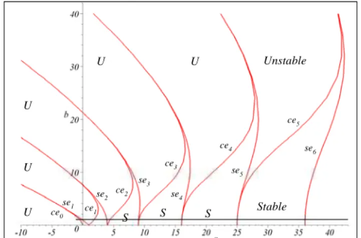
J. of the Braz. Soc. of Mech. Sci. & Eng. Copyright © 2008 by ABCM July-September 2008, Vol. XXX, No. 3 / 183 Stable Unstable S S S U U U U
U ce0
se1 ce 1
se2 ce2
se3 ce3 se4 ce4 se5 ce5 se6
Figure 1. Mathieu stability chart based on the numerical values, generated by (McLachlan, 1947).
Energy-Rate Method
The Energy-Rate method can be applied to the following general parametric differential equation:
( ) (
, ,)
0x+ f x +g x x t =
&& & (2)
where, f(x) is a single variable function, and g x,x,t
(
&)
is a smooth periodic time varying function with the following conditions.(
0 0)
0g , ,t = . (3)
(
) (
)
g x,x,t& + =T g x,x,t& (4)
Furthermore, the functions f and g can depend on finite sets of parameters. Equation (2) may be assumed as a model of a unit mass attached to a spring, acted upon by a non-conservative force
(
)
g x,x,t
− & . Introducing the kinetic, potential, and mechanical
energies for the system, 2
( ) / 2
T x& =x& , ( )V x =
∫
f x dx( ) , and ( ) ( )E=T x& +V x , we may transform Equation (2) to an integral of energy as follows:
(
)
(
)
2 1 ( ) ( ) , , 2 d dE E x f x x dt x g x x t
dt dt
⎛ ⎞
= = ⎜ + ⎟= − ⋅
⎝
∫
⎠& & & & & . (5)
The function E&= − ⋅x g x x t&
(
, ,&)
, which is equal to the time derivative of the mechanical energy of the system, represents the instantaneous rate of generated or absorbed energy by the applied force g x,x,t(
&)
. Instantaneous generation or absorption of energy depends on the value of parameters, time, x, and x&. If the overall value of the rate of energy in an excitation period is negative for a set of parameters and a nonzero response x(t), the response of the system shrinks along the path of x(τ), t< τ < +t T, and the amplitude of oscillation decreases. On the other hand, if the overall value of the rate of energy in an excitation period is positive for a set of parameters and a nonzero response x(t), then the response of the system expands along the path of x(τ), t< τ < +t T, and the amplitude of oscillation increases.We define an Energy-Rate function as an average of the integral of the energy rate:
(
)
0
0
1T 1
T
Edt x g x,x,t dt
T T
Γ =
∫
& =∫
&⋅ & . (6)The Energy-Rate function is zero for free vibration of a conservative system, as well as the steady state (T/n)-periodic response of the system (2). Equation (2) includes two parameters, a and b, so the parameter space is two-dimensional. The number of parameters determines the dimension of the parameter space. Determination of stability diagram is carried-out by finding the pairs of (a, b) located on the boundary of stable regions. For a steady state
T-periodic response, we pick a pair of (a, b) and integrate Equation
(2) numerically to evaluate Γ. If Γ>0 then, (a, b) belongs to an unstable region where energy is being inserted to the system. However, if Γ<0, then (a, b) belongs to a stable region in which energy is being extracted from the system. On the common boundary of these two regions, Γ=0, and (a, b) belongs to a transition curve.
Let us fix b and search for a on a transition curve such that its left hand side is stable and its right hand side is unstable. So, if a point (a, b) shows that Γ is less than zero, the point is in the stable region. In such a case, increasing a will increase Γ. On the other hand, if Γ is greater than zero, the point is in the unstable region so, decreasing a will decrease Γ. The Energy-Rate function Γ can be used as a scale for converging a to an appropriate value, such that
Γ becomes zero. Applying this procedure, we find a point on a transient curve with a stable region on the left and an unstable region on the right. Varying b by an increment and repeating the calculation, we will find another periodic point. The transient curve can be found when b is varied enough to cover the entire domain of interest. It is often useful to have a prior understanding of behavior of the system.
Reversing the strategy and searching for transient curves whose right hand side is stable and left hand side is unstable, completes the stability diagram of the system. This procedure can be arranged in an algorithm to be set up in a computer program, as follows:
Step 1 - set a
Step 2 - set b, equal to some arbitrary small value Step 3 - solve the differential equation numerically Step 4 - evaluate Γ
Step 5 - decrease / increase a, if Γ >0 / Γ <0 , by a small increment
Step 6 - the increment of a must be decreased if Γ(a )i × Γ(a )<0i-1
Step 7 - save a and b when Γ <<1
Step 8 - while b<bfinal , increase b and go to Step 3 Step 9 - reverse the decision in Step 5 and go to Step 1
An alternative method is to set a domain of interest in the parameter plane and then, evaluate Γ for the domain using a fine resolution. A dimensional matrix will be found for a two-parameter equation. Each element of the matrix would be the value of Γ for the associated pair of parameters. Using this matrix, a three-dimensional surface can be plotted to illustrate the Energy-Rate function. This plot shows the relative stability of different points in the parameter plane. Intersection of the surface with plane Γ=0 designates the transition curves, while the domain below it indicate stable regions, and the domain above this plane indicate instable regions. The accuracy of this analysis depends on the resolution in the parametric plane.
Second, it can be applied to both, small and large values of parameters. Third, the values of the parameters for a periodic response can be found faster and more accurately than in other methods. Fourth, application of the Energy-Rate method for detection of periodic solutions can be adjusted to detect any periodic response, not necessarily on the boundary of stable and instable regions. Fifth, the Energy-Rate function can be used as a gauge function to compare the relative stability of different points of parameter space.
The greatest disadvantage of perturbation methods is that they can usually be applied to very small values of the parameters. Also, the accuracy of the results of most asymptotic methods cannot be increased by increasing the degree of polynomials or the number of terms in the perturbed solution.
In the next section we apply the Energy-Rate method to the Mathieu equation and to forced Mathieu type equation to show that the Energy-Rate method provides much more accurate stability diagram as compared to perturbation methods.
Stability Diagram of Mathieu Equation
To show the applicability of the Energy-Rate method, Mathieu equation is examined as the first example. Mathieu equation is a well investigated equation, and because of its linearity, there exist some effective methods for finding its stability diagram. Transition curves of Mathieu equation are π and 2π-periodic. The analytic solution of the equation on transient curves are available and are called cosine and sine elliptic functions (Richards, 1983). The first three even and odd cosine and sine elliptic functions, ce2n , se2n , ce2n+1 , and se2n+1 are shown in Figure 1. The unstable tongues are bounded with two transition curves starting from integer roots of
2
a− =n 0, n=0, 1, 2, 3,…. It can be shown that although the odd order cosine and sine elliptic functions are not symmetric with respect to b, the overall stability diagram looks symmetric.
Since the parametric resonance of Mathieu equation happens in periods T and 2T, the bound of integral may be defined from zero to
2T to include T and 2T periodic solutions. The Energy-Rate function
for Mathieu Equation (1) would be a two-parameter equation.
( )
2(
)
0
1
2 2
2
a,b b x x cos( t ) dt
π
Γ = Γ = ⋅ ⋅ ⋅
π
∫
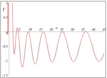
& (7)Consider a case in which b=1, then Γ is only a function of a. This function is plotted in Figure 2 using 10000 points in the interval 0<a<45. It can be seen that the curve Γ intersects the a axis exactly at the same points where the line b=1 intersects the transition curves of the Mathieu stability diagram (see Figure 1).
Evaluating Γ over a domain of a and b generates a three dimensional stability surface. Figure 3(a) displays the stability surface of Mathieu equation over the area 2− < <a 12 and
0< <b 12. Based on Energy-Rate method, wherever Γ is negative, Mathieu Equation (1) is stable, and wherever Γ is positive, it is unstable. The stability surface has been found by integrating over
T=2π. Therefore, the intersection of the stability surface with the plane Γ=0, indicates π or 2π-periodic curves, because a π-periodic function is 2π-periodic as well. Figure 3(b) depicts a top view of the stability surface. It also illustrates the intersection curves of the stability surface with plane Γ=0.
Γ
Figure 2. Plot of π for Mathieu equation as a function of a for b=1.
a
b
Γ
Figure 3(a). Stability surface of Mathieu Equation (1).
a b b
12
10
8
6
4
2
0
-2 0 2 4 6 8 10 12
Figure 3(b). 2π-periodicity curves of Mathieu Equation (1).
J. of the Braz. Soc. of Mech. Sci. & Eng. Copyright © 2008 by ABCM July-September 2008, Vol. XXX, No. 3 / 185 a
b 12
10
8
6
4
2
0
-2 0 2 4 6 8 10 12
Figure 4. 2π-periodicity curves of Mathieu Equation (1), intersection of the
stability surface and plane Γ =0.
Stability Diagram of A Forced Mathieu Type Equation
As a second example, forced vibration of a Mathieu type system will be studied in this section. Consider the following forced and parametrically excited equation:
( )
(
)
2( )
y+ + − β + βhy 1 2 2 cos 2rt y= β2 sin rt
&& & . (1)
which is the nondimensionalized governing equation of a linearized model of a micro-electro-mechanical system (Luo, 2002) (Jazar, 2006). The system is a cantilever resonator activated by an alternating electric field. Equation (1) is dependent on three independent parameters. Therefore the parameter space of the system is a three-dimensional r-β-h space. Assuming h=0, the
condition for parametric resonance, which states that n times of the forcing frequency is equal to twice of the natural frequency of the unforced system, would be 1 2− β =nr ,n∈N. Therefore, transition curves, if there is any, must start from r=1 / n,n∈N on the line β=0. The periodic curves corresponding to n=1 makes the
principal instability domain, if they are transition curves. Assuming a periodic solution, y n 0Y sin( nrtn )
∞ =
=
∑
+ ϕ , andapplying multiple scale perturbation method provides the following relationship for the periodic condition with Y0=0.
(
)
(
)
2 2 4 2 2
2 1
r 2 h 4 h 4h 1 2 4 , n N
2n
= − − β ± − − β + β ∈ . (2)
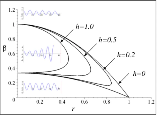
Traditionally, the periodic condition is used to determine the periodic curves in parameter plane r-β. The periodic curves need to be checked to determine if they are transition or splitting curves. The periodic curves (2) corresponding to n=1 are plotted in Figure 5
for different values of h. It is expected that two periodic curves
come out of r=1 and make the principal instability tongue. Time
response of the undamped system for selected points (r, β) =
(0.9, 0.1), and (1.2, 0.1), are found and shown in Figure 5. It is
concluded that Equation (2) are transition curves, and the region surrounded by curves coming out of r=1 is unstable. Figure (5) also
illustrates that the instability domain shrinks by increasing the dimensionless damping, h.
β
r
h=0
h=0.2
h=0.5
h=1.0
Figure 5. Transient curves and instability region for Equation (1).
Applying Poincare-Lindstad method provides the following equations for no damping transient curves will be found
2 4
1 1 r O( r )
β = − +
2 4 2
1 r
O( r )
3 3
β = − + (3)
which are in agreement with Equation (2) and Figure 5.
It must be mentioned that not only the curves derived from perturbation analysis are not necessarily transition curves, the stability behavior of the system is also questionable when parameters are close to a curve. Furthermore, we know that although Equations (2) and (3) might be used to determine the periodic curves and stability regions in r-β space around β=0, they cannot be used
to determine the global stability regions of the system. Defining the Energy-Rate function as follow:
( )
( )
(
)
2
2
0
2 / r
r
y sin rt hy y cos rt dt
π
′
Γ = β − − β
π
∫
& . (4)and applying Energy-Rate method provides an exact stability diagram. To present a better view of stability diagram, we study the system in 1/r-β plane instead of r-β plane. However, it is also possible to apply a transformation
rt
= τ
, and convert Equation (1) into the form:( )
(
)
2( )
y′′+2Hy′+ A+2B cos 2τ y=2B sin τ
where,
y′ =dy / rdτ, 2
2H =h / r ,
(
)
2A= − β1 2 / r , 2
B= β/ r .
Therefore, the Energy-Rate function may be defined as
( )
( )
(
)
2 2
0 2
*
y B sin rt Hy By cos d
π
′ ′
πΓ =
∫
− − τ τ.A three dimensional illustration of stability surface πΓ/ r is depicted in Figure 6(a) to provide a relative stability view. The stability surface is made by 5000 1000× points. The intersection of the stability surface with Γ=0 specifies the transition curves of the
by investigating Figures 6(a) or 6(c). It can also be determined by numerical solution of the equation for a sample point within each region.
A deep and an elevated regions are associated to strong stable and an unstable region: a stable region for large values of β around
r=1, and an unstable region corresponding to large values of β and
1/r. There is also an unstable region connected to 1/r=1 which is the
principal instability region that could be predicted by perturbation methods approximately.
β
1/r
πΓ
/r
Figure 6(a). Stability surface for the parametric Equation (1).
1/r
β
U
S
S
U
U
S
S
S
S
Figure 6(b). Stability diagram for the parametric Equation (1).
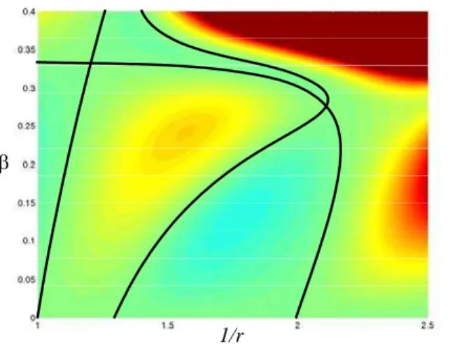
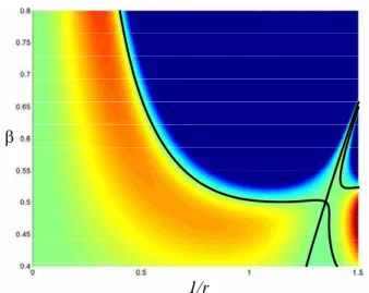
Because of the importance of the principal instability region, a magnified view of the stability surface for 0<β<0.4 and 1<1/r<2.5
is shown in Figure 7(a). A better view of the transition curves is depicted in Figure 7(b). A top view of the stability surface along with the transition curves are also shown in Figure 7(c) to highlight the stability characteristic of Figure 7(b). In order to better understand the behaviour of the system when parameters are around the principal instability region, time responses of the system for a few selected points in different regions are shown in Figure 8. The examined points are marked in Figure 7(b).
1/r
β
Figure 6(c). Top view of the stability surface for the parametric Equation (1) along with transition curves.
1/r
β πΓ/r
Figure 7(a). Magnification of stability surface at the principal instability region of the parametric Equation (1).
1/r
β U
S
U
U S
S
J. of the Braz. Soc. of Mech. Sci. & Eng. Copyright © 2008 by ABCM July-September 2008, Vol. XXX, No. 3 / 187 1/r
β
Figure 7(c). Top view of the stability surface of Equation (8) along with transition curves around the principal instability region.
Comparison of the results of perturbation analysis in Equation (9) or (10) with the results of Energy-Rate method is shown in Figure 9. From a design point of view, the strong stable region related to r≈1 and large values of β are important. This is probably the best area to set the parameters of the system governed by Equation (8). To clarify the boundary of the stable and unstable regions in this area, a three dimensional illustration of stability surface, and a two dimensional stability diagram are shown in Figures 10-12.
Y
t
h=0.0
β
=.24
1/r=1.5
β
=.13
1/r=1.8
β
=.37
1/r=2.4
β
=.15
1/r=2.45
β
=.25
1/r=1.0
Figure 8. Time response of the parametric Equation (8) for some points of the parameter plane.
1/r β
Perturbation method Energy-Rate method
Figure 9. Comparison of the result of perturbation and Energy-Rate method close to the principal instability region of Equation (8).
β
1/r πΓ/r
Figure 10. Magnification of stability surface around the strong stable region of the parametric Equation (8).
1/r β
S S
U U
S
1/r
β
Figure 12. Top view of the stability surface of the parametric Equation (8) along with transition curves around the strong stable region.
Conclusion
The Energy-Rate function, 0
(
)
Tx g x,x,t dt / T
⎡ ⎤
Γ =⎢⎣
∫
&⋅ & ⎥⎦ is used togenerate a three-dimensional stability surface for two parametric equations example. The value of the function can be determined numerically and compared to zero for a parametric equation such as
( ) (
, , , ,)
0x+ f x +g x x t a b =
&& & . The Energy-Rate method may be used to investigate the stability of the parametric equations. Procedure of searching for periodic curves in the parameter space is presented as an algorithm.
To validate the algorithm, it was applied to the Mathieu equation, and its stability chart was developed. The results are in agreement with a previously reported results. In the second example, the method was applied to a forced and parametrically excited equation, which is based on the model of a physical system. Multiple time scale, and Poincaré-Lindstad perturbation methods were applied and periodic curves for small values of parameters were found. The stability surface and stability diagram of the system
are also found by applying the Energy-Rate method. Three-dimensional illustration of stability surface shows a sense of relative stability of parameter plane. The intersection of a zero plane with stability surface determines the periodic and transition curves of the system. The procedure is sometimes time consuming, but it generates a more efficient and more accurate stability diagram.
References
Butcher E.A., and Sinha S.C., 1998, “Symbolic Computation of Local Stability and Bifurcation Surfaces for Nonlinear Time-Periodic Systems”,
Nonlinear Dynamics, 17, 1-21.
Butcher, E.A., and Sinha, S.C., 1995, “On the Analysis of Time -Periodic Nonlinear Hamiltonian Dynamical Systems”, ASME Design Engineering Technical Conferences DE 84-1, Vol. 3, part A, 375-386.
Guttalu, R.S., and Flashner, H., 1996, “Stability Analysis of Periodic Systems by Truncated Point Mapping”, Journal of Sound and Vibration, 189, 33-54.
Hayashi, C., 1964, Nonlinear Oscillations in Physical Systems, Princeton.
Iwanowski, E.R.M., 1965, “On the Parametric Response of Structures”,
Applied Mechanics Review, 18(9), 699-702.
Jazar, Reza N., 2004, “Stability Chart of Parametric Vibrating Systems, Using Energy Method”, International Journal of Nonlinear Mechanics, 39(8), pp. 1319-1331.
Jazar, Reza N., 2006, “Mathematical Modeling and Simulation of Thermoelastic Effects in Flexural Microcantilever Resonators Dynamics”,
accepted for publication in the Journal of Vibration and Control.
Luo, A. C. J., 2002, “Chaotic Motion in the Generic Separatrix Band of a Mathieu-Duffing Oscillator with a Twin-Well Potential,” Journal of Sound
and Vibration, 248(3), 521-532.
McLachlan, N. W., 1947, Theory and Application of Mathieu Functions, Clarendon, Oxford U. P., Reprinted by Dover, New York, 1964.
Richards, J. A., 1983, Analysis Periodically Time Varying Systems, Springer-Verlag, New York.
Sinha S.C., and Butcher E.A, 1997, “Symbolic Computation of Fundamental Solution Matrices for Linear Time-Periodic Dynamical Systems”, Journal of Sound and Vibration, 206(1), 61-85.
Van der Pol, B.,, and Strutt, M.J.O., 1928, “On the Stability of the solution of Mathieu’s Equation”, The Philosophical Magazine, vol. 5, p. 18.