Miguel Vaz Júnior
Emeritus Member, ABCM [email protected]Paulo Sergio B. Zdanski
[email protected] State University of Santa Catarina - UDESC Department of Mechanical Engineering 89223-100 Joinville, SC, Brazil
Eduardo Luís Gaertner
[email protected] Empresa Brasileira de Compressores S.A. Rua Rui Barbosa, 1020 89219-901 Joinville, SC, Brazil
Aspects of Finite Element and Finite
Volume Equivalence and a Posteriori
Error Estimation in Polymer Melt Flow
In this work, aspects of discretization errors associated with finite volume (FV) and equivalent finite element (FE) modelling strategies are discussed within the framework of polymer melt flow. The computational approaches are based on the generalized Newtonian model in conjunction with Cross constitutive equation. The numerical examples illustrate one and two-dimensional fluid flows, in which the latter is discretized using structured quadrilateral elements / volumes. A study on the best strategy to compute non-linear viscosities at control volume boundaries is also presented for FV. Based on well established a posteriori error estimation techniques, it is demonstrated that, in this class of problems, FV discretization errors and differences between FE and FV solutions are greatly affected by the scheme used to compute the FV non-linear coefficients at the control volume surfaces. Simulations for rectangular channels show that FE yields smaller global errors then FV for velocity and temperature solutions.Keywords: polymer melt, finite volumes, finite elements, error estimation
Introduction
1In the last twenty years, commercial software packages aiming
at simulation of polymer processing, such as extrusion and injection moulding, have been steadily developed, most of which able to handle applications ranging from common household objects to complex aerospace components. Due to the complexity of such problems, most commercial programs attempt to combine practical rheological models with approximate computational modelling techniques. Such approach has hampered more comprehensive studies on the polymer behaviour and further understanding of the interaction of the problem parameters. However, in the last years, the literature shows an increasing attention in the simulation of polymer processing operations using more elaborate material modelling. For instance, Carreau and Cross constitutive equations
have been used to study several aspects of injection moulding. The former was adopted to describe error estimation associated with finite elements (Bao, 2002; Fortin et al., 2004), whereas the latter was used to study the effects of viscous dissipation and axial heat conduction (Zdanski and Vaz Jr., 2006) and error assessment (Vaz Jr. and Gaertner, 2004, 2006). The present work addresses some modelling aspects of polymer melt flow using finite volumes (FV) and finite elements (FE) schemes, such as computation of the FV non-linear coefficients at the control-volume surfaces, approximation between FE and FV solutions and FV and FE error estimation. The numerical examples illustrate one and two-dimensional fluid flows, in which the latter is discretized using structured quadrilateral elements / volumes.
Nomenclature
e = error in the Energy norm
h = mesh size
H =channel height
J2 = second invariant of the rate of the shear strain tensor
k =thermal conductivity
kp = power-law consistency index
L =channel length
n = power-law index
p = order of the discretization error
Paper accepted April, 2008. Technical Editor: Olympio Achilles de F. Mello.
p
~ = estimated order of the discretization error
P = pressure
q = polynomial order of the approximation
r = mesh refinement ratio, r = h2/ h1and h2 > h1 R2 = coefficient of determination
T = temperature
Tw = channel wall temperature
w = velocity
W = channel width
Greek Symbols
H = Richardson or exact error
K = shear viscosity
K0 = Newtonian viscosity
Ȗ = rate of the shear strain tensor J = equivalent shear strain
O = material parameter
U = specific mass
W = equivalent shear stress, W KJ
\ = effectivity index Subscripts
E Energy norm
h variable at Gauss points
h1 variable or Richardson error for mesh h1
R Richardson estimate
RMS Root Mean Square
T temperature
w velocity
Superscripts
a analytical or exact solution FE finite element solution FV finite volume solution
w velocity
Governing Equations and Polymer Rheology
The physics of polymer melts in injection moulding suggests that fluid flow is governed by the shear viscosity, which makes possible to use the generalised Newtonian model,
Ȗ
where IJ is the shear stress tensor, K is the shear viscosity and Ȗ is the rate of strain tensor. In such problems, viscosities are related to temperature, T, and the second invariant of the rate of strain tensor, J2, so that
2 / 1 2
/ 1
2 (1/2Ȗ:Ȗ)
J
J , (2)
in which J is the so-called equivalent shear rate. The general
approach is based on the coupled solution of the momentum and energy equations, which, for fully developed fluid flow, can be written as
>
@
z P w T
w w
) , (
divK J and div
>
kT@
WJ 0 , (3)where w is the velocity, wP/wz is the pressure gradient, k is the thermal conductivity, WJ represents the viscous heating and W is
the equivalent stress. It is interesting to mention that studies using velocity and temperature fully coupled approaches associated with polymer melt flow based on realistic material modelling are still scarce (the reader is referred to Vaz Jr. and Zdanski (2007) for further discussions on the issue). Notwithstanding, a number of works based on formulations similar to Eq. (3) have been recently published, such as Syrjälä (2002), Hashemabadi et al. (2003), Pinarbasi and Imal (2005) and Vaz Jr. and Gaertner (2006).
In this work, shear viscosity is described by both the power law
andCross constitutive models. Polymer melts approach the power law behaviour for large shear rates, in which
1
n p kJ
K , (4)
where kp is the consistency parameter and n is the power law index.
Due to inexistence of analytical solutions for Cross equation, some error analyses have only been performed for power-law fluids (kp =
18,332.63 and n = 0.36043). The Cross constitutive equation is
adopted to describe the commercial polymer Polyacetal POM-M90-44 used in the last numerical example. This polymer has shown strong temperature dependency, so that
>
@
1 ( ) 0) ( 1
) (
, nT
T T
T
O J
K J
K
, (5)
in which
¸ ¹ · ¨ © §
¸ ¹ · ¨ © §
¸ ¹ · ¨ © §
T c c T n
T b b T
T a a T
2 1
2 1
2 1 0
exp ) (
exp ) (
exp ) (
O K
, (6)
where a1 = 0.022603 Pa.s, a2 = 5,003.01 K, 1 1.6425 106
u
b ,b2 =
3,901.0 K, c1 = 1.3574 and c2 = 653.73 K (Herrmann, 2001). The
specific mass and thermal conductivity used in the simulations are U
= 1143.9 kg/m3 and k = 0.31 W/m K, respectively.
Numerical Modelling
FE and FV Approximations
The FE method is based on Galerkin weighted residuals and assumes that the exact solution can be interpolated from C0
-continuous shape functions. The FE equations have been approximated using the classical four-noded isoparametric elements and the Gauss quadrature (Zienkiewicz and Taylor, 1994). The FV discretization procedure applies the conservation laws to discrete, non-overlapping control volumes (Ferziger and Periü, 1999). The FV equations are approximated using linear interpolation functions and assume uniform shear rate, viscosity and thermal conductivity over the control volume surfaces.
Remark 1: It is well known that, in self-adjoint problems, the
finite element method associated with Galerkin weighting provides an optimal approximation and, therefore, yields more accurate results. Moreover, Idelsohn and Oñate (1994) demonstrate that, for
linear advective-diffusive problems, a generally non-symmetric FV
characteristic matrix can be transformed into an identical FE “stiffness” matrix when linear triangles with a lumped mass matrix are used in both methods, the proportional vertex centred scheme is employed in FV and the source terms are constant. The contrast between using linear diffusive coefficients (e.g. viscosities) and the material nonlinearity of the present work precludes a straightforward extension of Idelsohn and Oñate's (1994) conclusion to polymer melt flows. Furthermore, FE and FV compute shear rates and viscosities at different locations. The former evaluates J and K
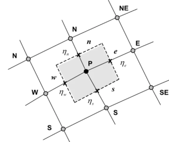
at the Gauss points, as illustrated in Fig. 1, and the latter at the control volume boundaries, as depicted in Fig. 2. In spite of such issues, the first two numerical examples demonstrate that the scheme to compute viscosities at the control volume surfaces dictates FE and FV solution equivalence.
Figure 1. FE four-noded element: viscosity and shear strain rate computed at Gauss points.
Figure 2. Structured two-dimensional finite volume mesh: viscosity and shear strain rate computed at the control volume surfaces.
n
s e
s K n K
e K
w Kx w
S N
E
W N
NE
S
SE P
x x x
N3 N4
N1 N2
3
K
1
K
2
K K4
x x
FV Interface Quantities
The scheme to evaluate shear strain rate, viscosities and temperatures at control-volume surfaces in FV has shown of paramount importance in this class of problems due to its high material nonlinearity. Strategies can be divided into three groups: (i)
computation of shear rates and viscosities at nodes followed by interpolation at the control-volume surfaces; (ii) computation of
shear rates at nodes followed by interpolation over the volume interfaces and evaluation of the corresponding viscosities and (iii)
computation of the shear rates directly at the control-volume surfaces followed by evaluation of the corresponding viscosities. The following paragraphs summarise some of the methods associated with the strategies previously mentioned. For the sake of clarity, the approximations are presented for surface “e” of a
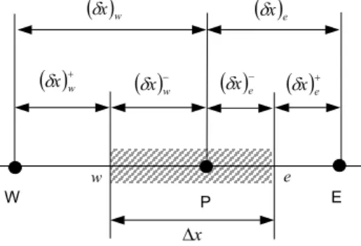
one-dimensional control volume, as illustrated in Fig. 3.
P
w x G
e x G
w
Gxw
w x
G
e x
G
e x G
e
W E
x '
Figure 3. One-dimensional control volume and neighbouring nodal points.
The most widely used schemes to estimate diffusivity properties at the control volume surfaces are based on the harmonic mean, advocated by Patankar (1980), and a linear interpolation between nodesP and E, which, in this case, can be represented, respectively, as
e E e PP E e
f
f K K
K K K
1 , and Ke feKP
1feKE, (7)where fe
e
Gxe/Gx. Alternatively, the
Kirchhoff approximation,
based on the namesake transformation, was proposed by Voller and Swaminathan (1983) to evaluate discontinuous thermal conductivity, which, in the present case, is used to approximate viscosities as
J J K J J
K J
J
d E
P P E
e ³
1
. (8)
In a recent comparative work for one-dimensional problems, Liu and Ma (2005) proposed a different method to compute nonlinear thermal conductivity at volume interfaces that yields better results then the harmonic mean. Based on Liu and Ma's (2005) concept, the shear rate at the volume surfaces are estimated first, followed by computation of the corresponding viscosity,
e EP e
e fJ f J
J 1 and
e e e K J
K . (9)
This work proposes computation of J at the control-volume
(CV) surfaces directly from velocities located at neighbouring nodes. For one-dimensional problems, the equivalent shear rate is reduced to
e E P
e e
x w w x w
G
J ¸
¹ · ¨ © § w w
and
e e e K J
K , (10)
where wE and wP are nodal velocities. Computation of viscosities
follows Eq. (10)b. Despite the additional care required on programming the algorithm for two and three-dimensional problems, one should note that the direct evaluation of the shear rate at the control-volume surfaces is based on central derivatives, thereby yielding a second-order approximation to the shear rate. This work presents an error assessment of the methods described by Eqs. (7)-(10).
Viscosity computation using Eq. (5) also requires temperatures at volume surfaces. In case of collocated meshes for velocities and temperatures, interface temperatures can be easily estimated using a linear interpolation between the corresponding points (Liu and Ma, 2005), which, in the one-dimensional example, one obtains
e E Pe
e fT f T
T 1 . (11)
Error Estimation
Despite the increasing number of works concerned with injection moulding, error estimation using the generalised Newtonian model, especially associated with finite volumes/finite differences, has been rarely mentioned in the literature. Bao (2002) proposed an error estimation scheme for finite elements based on a discrete Babuska–Brezzi inf-sup condition. An error estimator based on the second derivative of velocities for FE solutions was used in conjunction with an h-adaptive procedure by Fortin et al. (2004). Application of Richardson extrapolation (Richardson, 1910) and error norms (Zienkiewicz and Zhu, 1987) to estimate discretization errors in polymer melt flows were also described by Vaz Jr. and Gaertner (2004, 2006). The present work emphasises discretization errors of FV solutions and their equivalence to FE approximations based on Richardson extrapolation and analytical solutions for simple constitutive relations. Error in the Energy norm associated with FE is also summarised in the following sections.
Richardson Extrapolation
Richardson (1910) ascertained that a higher order solution could be achieved by assuming that the “exact” solution is described as
1 1 1
1 1 1
p p
h h h
exact I H I Dh Oh
I x x x x (12)
where Iexact and Ih1 are, respectively, “exact” and discrete solutions
at a given point x, Hh1is the discretization error, h1 is the mesh size, D is a constant and p is the error order. The exact order of the discretization error is hardly known a priori, which recommends use of an estimate ~p. Therefore, Hh1and p
~ can be determined by
assuming (and verifying) asymptotic convergence (Oberkampf and Trucano, 2002) and by applying Eq. (12) to three nested meshes, h1,
h2, and h3, which, for a constant refinement ratio, r, yields
1
~ 2
1 1
1
#
hp h
h exact h
r I I I I
HI , (13)
1 2 2 3 log log ~ 1 2 2 3 h h h h r r p h h h h ¸ ¸ ¹ · ¨ ¨ © § I I I I (14)
where h3 > h2, > h1. The global measure is defined by the error norm
as ¦ ¦ ¸¸ ¹ · ¨¨ © § R R N k k p h h N
k h k h r 1 2 ~ 1 2 2 1 2 1 1 1 I I HI I I
H (15)
where NR represents the number of nodes coinciding to meshes h1,
h2, and h3, HhI1 is the local error and I corresponds to either nodal
velocities, I = w, or nodal temperatures, I = T. Although the technique described previously can handle only uniform meshes, extensions have also been developed for non-uniform grids (Ferziger and Periü, 1996) and multi-dimensional transient problems (Marchi and Silva, 2005).
A Posteriori Projection / Smoothing Technique
Error estimation has become an important issue in computational mechanics since the late seventies when Babuška and Rheinboldt (1978) proposed a posteriori error estimates for the
finite element method using norms of Sobolev spaces. The topic gained momentum when Zienkiewicz and Zhu (1987) introduced error estimates based on post-processing techniques of the finite element solutions. Due to its relative simplicity, the original Zienkiewicz and Zhu’s scheme has been extended to a wide spectrum of applications, ranging from linear solid mechanics to the highly non-linear metal forming problems. This strategy was also employed successfully by Wu et al. (1990) for solving the incompressible (Newtonian) Navier-Stokes fluid flow around a cylinder using an error estimate based on the Energy norm. The present work summarizes application of the Energy norm,
>
@
:|³>
@
: ³ : : d IJ IJ d IJIJ h h h h h h
E J J J J
- * *
-2
e , (16)
in which W and J are the “exact” values of the equivalent stress and equivalent shear rate, respectively, and the subscript h indicates the corresponding finite element approximations. The standard post-processing of the finite element solution provides the equivalent shear rate, Jh, and equivalent shear stress, Wh, at the integration
points. The “exact” solution is determined based on Zienkiewicz and Zhu's (1987) concept, which comprises (i) extrapolation from Gauss points, Wh and Jh, to nodes, (ii) followed by an interpolation
back to the integration points, *
h
W and *
h
J . Additional details on the strategy to compute errors in the Energy norm are presented in Vaz Jr. and Gaertner (2004).
The previous scheme has the advantage of computing the error estimate using only one mesh, being intrinsically associated with the finite element method. Despite its extensive use in almost every field of computational mechanics, this technique has the disadvantage of estimating errors based on secondary measures (stresses and strain rates). It is worthy to emphasise that research on error estimation for polymer melt flow is still in its infancy and further investigation to assess accuracy and applications to complex flows are recommended.
Numerical Examples
A suitable quantification of the solution accuracy is crucial to establish confidence in the numerical model. The instinctive assumption that by refining the mesh one obtains more accurate results is not always true. Therefore, error assessment is a fundamental step during the development of a numerical model. This section is divided into tree parts: (i) assessment of the schemes
used to evaluate viscosities at control-volume surfaces for FV, (ii)
evaluation of Richardson errors for FE and FV and their equivalence, and (iii) discretization errors for polymer melt flow in thick channels. Analyses (i) and (ii) aim at assessing the accuracy degree of the approximations by comparing analytical solutions for isothermalpower-law fluid flow in plane channels and rectangular channels with large aspect ratios. Case (iii) uses the Cross
constitutive equation and addresses velocity and temperature fully coupled solutions.
Isothermal Power-Law Fluid Flow in Plane Channels
This section discusses solution accuracy in association with different schemes to compute viscosities at the control-volume surfaces. Global and local errors are evaluated under the framework of isothermal power-law fluid flow in plane channels. Estimates using Richardson extrapolation have also been studied aiming at establishing the spatial error order. The analytical solution for fully developed fluid flow between parallel plates can be readily derived as » » » ¼ º « « « ¬ ª n n a a H H y n n w y w 1 2 / 2 / 1 1 1 2
, (17)
in which a
w is the mean velocity, n is the power-law index, H is the
gap thickness and y is measured from the lower plate. Global RMS
velocity errors associated with analytical solutions (exact errors), w
RMS
H , and Richardson extrapolation, w
RMS R,
H , are defined,
respectively, as
1/2 1 2 1 »¼ º «¬ ª ¦N i a i i wRMS w w
N
H and
2 / 1 1 2 , , 1 » ¼ º « ¬ ª ¦R N
k Rk R w RMS R N I H
H , (18)
where N is the number of nodes, and NR and HRw are Richardson's
number of points and local errors respectively.
Simulations have been performed for channel gap thickness H =
2; 4 and 8 mm, mean velocities a
w = 1.0 to 10.0 cm/s and
normalised mesh sizes ranging from h/H = 0.003125 to 0.1. In order
to avoid the typical power-law singularity at the channel centre,
harmonic and linear interpolation (Eq. 7), and Kirchhoff (Eq. 8)
viscosity means require even node numbers, whereas linear interpolation of J at the control-volume surfaces (Eq. 9) and direct shear rate computation at surfaces (Eq. 10) require odd node numbers. Furthermore, Eq. (7) and Eq. (8) demand computation of
J at the channel surfaces, which in turn, require velocity
derivatives at such locations. The latter has been examined using first (two-point) and second (three-point) order approximations.
9879 . 1 4619
.
1 ¸
¹ · ¨ © §
H h wa w
RMS
H [cm / s] , (19)
fordirect shear computation (Eq. 10). In statistics, the quality of the
curve fit is generally measured by the coefficient of determination,
R2, which ranges from 0 (no actual co-relation between the original data set and the best-fit curve) to 1.0 (the variability between the original data and the fitted equation is very small). In this case, the simulations have shown that the coefficient of determination approximates R2 = 1.0 for the curve represented by Eq. (19). A more
formal error analysis is outside the scope of the present work. However, errors associated with the analytical solution can be
alternatively expressed using the L2-norm, so that
0003 . 2 0003 . 2
2
2 1.498
h H
L a L
a
w w
w .
It is relevant to mention that shear rates computed using direct shear computation (Eq. 10) have provided absolute global errors
around 7.5 times smaller than the scheme based on Eq. (9), i.e.,
linear interpolation of the shear rate at FV surfaces followed by computation of viscosities. The other methods used to evaluate viscosity at volume interfaces yield even worse solutions (the errors provided by linear interpolation, Kirchhoff mean and harmonic mean are, respectively, 17, 10 and 9 times larger then the errors computed when using direct shear computation).
0.0 1.0 2.0 3.0 4.0 5.0 6.0 7.0
0.0 1.0 2.0 3.0 4.0
y [mm]
w [
c
m
/s
]
Analytical Solution Direct shear (7 nodes) Interpolate shear (7 nodes) Kirchhoff (8 nodes) Harmonic (8 nodes) Linear (8 nodes)
Figure 4. Isothermal power-law fluid flow in plane channels: FV local velocities for H = 4 mm and wa = 5.0 cm/s.
1.0E-06 1.0E-05 1.0E-04 1.0E-03 1.0E-02 1.0E-01 1.0E+00
0.001 0.010 0.100 1.000
Mesh size h [mm]
G
lo
b
a
l R
M
S Er
ro
r [
c
m
/s
]
Linear Kirchhoff Harmonic Interpolate shear Direct shear
Figure 5. Isothermal power-law fluid flow in plane channels: FV global
RMS errors for H = 4 mm and wa= 5.0 cm/s.
An alternative appraisal of the discretization order for solutions using Eq. (9) (interpolate shear) and Eq. (10) (direct shear) has
been performed based on Richardson extrapolation. Eight nested meshes with a constant refinement radio r = 2 have been used (h / H
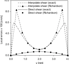
= 0.00078125, 0.0015625, 0.003125, 0.00625, 0.0125, 0.025, 0.05 and 0.1). Both schemes have shown monotonic rate of convergence and spatial error orders ~p|2.0. Local and global RMS errors are presented in Fig. 6 and Fig. 7 for a gap thickness H = 4 mm using the exact and Richardson definitions (Eq. 18). In case of direct shear computation (Eq. 10), errors calculated using Richardson
extrapolation render very close approximations to those determined based on the analytical solution. A somewhat close solution was also obtained for viscosities computed using linear interpolation of the shear rate (Eq. 9). Table 1 presents results for global RMS velocity errors corresponding to Figure 7. The accuracy of
Richardson estimates is defined by the effectivity index,
w RMS R w RMS /H ,
H
\ , which is also shown in Table 1.
0.0 2.0 4.0 6.0 8.0 10.0
0.0 1.0 2.0 3.0 4.0
y [mm]
Lo
c
a
l er
ro
rs
x
1
00 [c
m
/s
]
Interpolate shear (exact) Interpolate shear (Richardson) Direct shear (exact) Direct shear (Richardson)
Figure 6. Isothermal power-law fluid flow in plane channels: FV local errors (exact and Richardson) for velocities (H = 4 mm and wa = 5.0 cm/s).
1.0E-06 1.0E-05 1.0E-04 1.0E-03 1.0E-02 1.0E-01 1.0E+00
0.001 0.010 0.100
Mesh size h [mm]
G
lo
b
a
l R
M
S
E
rro
r [
c
m
/s
]
Interpolate shear (Richardson) Direct shear (Richardson) Interpolate shear (exact) Direct shear (exact)
Figure 7. Isothermal power-law fluid flow in plane channels: FV global
Table 1. Isothermal power-law fluid flow in plane channels: FV global RMS errors (exact and Richardson) in [cm/s] and the effectivity index, <.
Shear interpolation (Equation 9) Direct at the CV surfaces (Equation 10)
Mesh size
h / H Exact Richardson
Effectivity
index Exact Richardson
Effectivity index 0.100000 3.42710E-02 4.12830E-02 1.2046 4.81393E-03 4.64408E-03 0.9647 0.050000 8.86808E-03 9.89895E-03 1.1162 1.21084E-03 1.18881E-03 0.9818 0.025000 2.25690E-03 2.39548E-03 1.0614 3.03644E-04 3.00840E-04 0.9908 0.012500 5.69361E-04 5.87481E-04 1.0318 7.60304E-05 7.56742E-05 0.9953 0.006250 1.42991E-04 1.45321E-04 1.0163 1.90250E-05 1.89766E-05 0.9975 0.003125 3.58331E-05 3.61229E-05 1.0081 4.68924E-06 4.80745E-06 1.0252
It is important to note that the discretization errors have also been evaluated for second-order approximations of the velocity derivatives at the channel boundaries (i.e. using three nodal points). The issue is relevant only for cases which require computation of J
at nodal points. However, simulations have shown only limited
improvement for such cases, with direct shear computation
rendering global RMS errors 4.2, 4.9, 5.7 and 8.7 times smaller then the Kirchhoff mean, linear interpolation of viscosities, harmonic mean and linear interpolation of the shear rate, respectively.
Furthermore, it has been found that solutions using linear interpolation of the shear rate could not achieve monotonic rate of convergence
Remark 2: In all cases analysed, the direct shear computation at control-volume surfaces yields markedly smaller errors then the others schemes. Moreover, the numerical model based on Eq. (10) has presented monotonic rate of convergence with error orders close to 2.0. Use of second-order approximation of the velocity derivatives at the channel boundaries could not effectively improve solutions for schemes based on computation of shear rates at nodal points.
Figure 8. FE and FV approximations: local velocities for a mesh 90 x 6 elements/volumes.
FE and FV Isothermal Power-Law Fluid Flow in Rectangular Channels
This section addresses aspects of FE and FV simulation of isothermal power-law fluid flow in rectangular channels for large channel width / height, W / H, ratios (two-dimensional solutions approximate plane channels by disregarding the corner effect). This geometry makes possible to compare FE and FV results with
analytical solutions over the central line. Following the best approach determined in the previous section for FV, the shear rate is computed directly at the control-volume surfaces from neighbouring nodal velocities. The section presents results for a channel width W
= 300 mm, channel height H = 4 mm and mean velocities, a w ,
ranging from 1 to 10 cm/s. Five nested meshes (30 x 2, 60 x 4, 120 x
8, 240 x 16 and 480 x 32 elements) with constant aspect ratio, hx / hy
= 5, and refinement ratio, r = 2, have been used to estimate Richardson errors.
Figure 8 presents local velocities for wa = 1.0, 5.0 and 10.0
cm/s, from which one cannot visually distinguish FE from FV solutions. Global RMS errors computed from analytical solutions and Richardson estimates are shown in Fig. 9 (Eq. 18). Both schemes have shown monotonic rate of convergence and spatial error orders ~p|2.0. A direct relation between the FE and FV velocities can be established by using relative differences associated with the corresponding FE solutions and based on mesh size. The maximum relative differences, max
r
e , take place at the channel centre
and a curve-fit procedure (R2 = 0.9931) yields
444 . 1
max max 0.00033624
h w
w w
e FE
FV FE
r
(20)
for wa[1.0,10.0] cm/s, where wFE and
wFV are FE and FV local velocities respectively. Alternatively, FV and FE differences can
also be expressed using the Lf–norm as
444 . 1
0.00033624 h
L FE L
FV FE
f f
w w
w .
0.001 0.01 0.1 1
0.1 1.0
"y" mesh size [mm]
G
lobal
R
M
S
E
rr
or
[c
m
/s
]
FV - Richardson
FV - Exact
FE - Exact
FE - Richardson
Figure 9. FE and FV approximations: local velocities for a mesh 90 x 6 elements/volumes.
Remark 3: Despite the nonlinearity of the problem and differences on the scheme to compute viscosities, as discussed in
Remark 1, the present results show that for isothermal power-law
0.0 2.0 4.0 6.0 8.0 10.0 12.0 14.0
0.0 1.0 2.0 3.0 4.0
y [mm]
w [
c
m
/s
]
FE FV
a
w =10 cm/s
a
w =5 cm/s
a
fluids and fully developed flows, to a certain extent, an equivalence (a direct relation between both solutions can be establish and differences are sufficiently small and consistently quantifiable) can be ascertained between FE and FV methods only when the FV approximation computes shear rates directly at the control-volume surfaces.
Polymer Melt Flow in Thick Channels
This section summarises some aspects regarding error estimation using the Cross constitutive relation associated with fully-coupled momentum and energy equations. The reader is referred to Vaz Jr. and Gaertner (2006) for further details. The simulations assume uniform wall temperature, Tw = 493 K, and a
constant pressure gradient 'P/L = 44 MPa/m, and results are presented for a channel 5 x 5 mm. Seven nested meshes (2 x 2, 4 x 4,
8x 8, 16 x 16, 32 x 32, 64 x 64 and 128 x 128 elements / volumes)
with constant aspect ratio, hx / hy = 1, and refinement ratio, r = 2,
have been used to estimate Richardson errors.
The simulations show that the largest relative differences between FE and FV solutions for velocities are found, regardless the mesh size and H / W ratios, on the closest interior node to the
channel corners, decreasing subsequently towards the centre (from %
0 . 2
~ near the corner down to ~0.2% at the centre). This
behaviour can be credited to the differences on the strategies to compute viscosities for FE and FV (see Figs. 1 and 2). Contrary to the first two examples, in this case, viscosity requires computation of temperatures at the Gauss points (FE) and control-volume surfaces (FV). The former interpolates temperatures from nodal points using the shape functions, whereas the latter uses linear interpolation similar to Eq. (11).
The local error distributions for velocities based on Richardson extrapolation are illustrated in Figs. 10 and 11 for FE and FV, respectively. As discussed previously, local Richardson errors are computed using three nested meshes, which, in this example are
64 64
1 x
h , h232x32 and h316x16 elements /
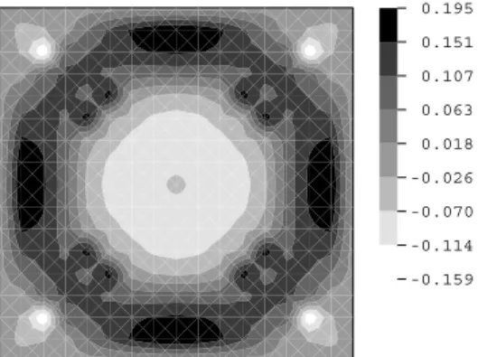
volumes. It is interesting to note that errors follow quite distinctive patterns for FE and FV solutions. The former shows large errors near the walls, as illustrated in Fig. 10, whereas the latter follows a more conventional pattern, always yielding maximum errors at the channel centre, as depicted in Fig. 11. Similar FE and FV error distributions have been observed for temperatures, which reach maximum values at the channel centre (FE solutions present smaller Richardson errors than FV ones).
0.195
0.151
0.107
0.063
0.018
-0.026
-0.070
-0.114
-0.159
Figure 10. Finite elements: local Richardson errors for velocities, wu101
h
H [mm/s], corresponding to a mesh 64 x 64 elements.
Despite the fact that FE solutions provide smaller Richardson errors than FV, the coupled character of the problem and the high material nonlinearity, allied to the scheme of computing shear rates
and viscosities, hinder a smooth distribution of error orders over the problem domain. Solution shows points of high convergence rates (~p|5) close to points of virtual divergence (~p|0.6) near the corners, which recommends greater care when using Richardson extrapolation in association with finite elements for this class of problems. However, despite the hindrances, this estimate becomes attractive due to its capacity to evaluate errors directly from primal variables. Contrastingly, the FV velocity and FE and FV temperature solutions present a smooth distribution of convergence orders over the problem domain (~p|2).
4.07
3.56
3.05
2.54
2.04
1.53
1.02
0.51
0.00
Figure 11. Finite volumes: local Richardson errors for velocities, wu101
h
H [mm/s], corresponding to a mesh 64 x 64 volumes.
Local error estimate for FE solutions using the Energy norm is illustrated in Figure 12 for a 64 x 64 mesh. It can be observed that
error distribution follows a somewhat similar pattern presented by the Richardson estimate shown in Figure 10.
3.35
2.98
2.62
2.26
1.89
1.53
1.16
0.80
0.43
Figure 12. Local error for the FE solution computed using the Energy norm, u103
E
e , for a mesh 64 x 64 elements.
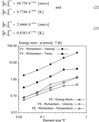
Remark 4: Figure 13 presents global convergence curves for both FV and FE Richardson extrapolation (Eq. 15) and FE Energy norm (Eq. 16). The literature indicates that, in the absence of singularities, for linear analysis of solid materials and Newtonian fluids (Zienkiewicz and Taylor, 1994), the global discretization error using the classical FE norms is proportional to hq, where h is
the element size and q is the polynomial order of the approximation.
This example uses linear elements (q = 1) and simulations show that
the convergence rate exhibited by the Energy norm follows similar rule, so that
9926 , 0 0211 .
2 h
E
Richardson error norms for FV and FE solutions have also shown convergence rates similar to the Energy norm, respectively represented as
] K [ 7746 . 8
] mm/s [ 759 . 69
0049 . 1
1620 , 1
1 1
h h
FV
T h
FV
w h
H H
and (22)
] K [ 8383 . 0
] mm/s [ 4466 . 2
7944 , 0
0328 , 1
1 1
h h
FE
T h
FE
w h
H H
. (23)
Figure 13. Global FE and FV errors for velocities and temperatures computed using Richardson extrapolation, and the Energy norm for the FE solution.
It is worth noting that hq is associated with the asymptotic rate
of convergence, defined as a global measure and computed over the problem domain, whereas hp is related to the order of the scheme,
calculated locally at the nodes. The former estimates global discretization errors and the latter approaches local approximation errors.
Concluding Remarks
This work addresses aspects regarding FV and FE approximations and error estimation strategies for polymer melt flow in closed channels. The governing equations are solved using both the FE and FV methods in association with linear quadrilateral elements/volumes and structured meshes. The power-law viscosity is used to assess solution convergence and accuracy, whereas the Cross constitutive equation is used in conjunction with the temperature-velocity fully coupled solution.
It has been demonstrated that the scheme to evaluate shear rate and viscosities at control-volume surfaces determines the error magnitude of FV solutions. The smallest errors have been achieved by computing the shear rate directly at the volume surfaces. It has also been shown that this scheme makes possible to establish certain equivalence between FV and FE solutions. This work has also addressed some aspects of solution accuracy and convergence using error estimates based on Richardson extrapolation and Energy norm for FE approximations of fully-coupled solutions. Some care should be taken when using Richardson estimates in association with FE owing to the smoothness of the error order distributions. However, it
has been observed that FE Richardson errors are substantially smaller then their FV counterparts.
References
Babuška, I. and Rheinboldt, W.C., 1978, “A posteriori error estimates for the finite element method”, International Journal for Numerical Methods in Engineering, Vol. 12, pp. 1597-1615.
Bao, W., 2002, “An economical finite element approximation of generalized newtonian flows”, Computer Methods in Applied Mechanics and Engineering, Vol. 191, pp. 3637-3648.
Ferziger, J.H. and Periü, M., 1999, “Computational Methods for Fluid Dynamics”, 2nd edn., Springer-Verlag, Heidelberg, 389 p.
Ferziger, J.H. and Periü, M., 1996. “Further Discussion of numerical errors in CFD”, International Journal for Numerical Methods in Fluids, Vol. 23, pp. 1263-1274.
Fortin, A., Bertrand, F., Fortin, M., Chamberland, É., Boulanger-Nadeau, P.E., Maliki, A.E. and Najeh, N., 2004, “An adaptive remeshing strategy for shear-thinning fluid flow simulations”, Computers and Chemical Engineering, Vol. 28, pp. 2363–2375.
Hashemabadi, S.H., Etemad, S. Gh., Golkar Naranji, M.R. and Thibault, J., 2003, “Laminar flow of non-newtonian fluid in right triangular ducts”,
International Communications in Heat and Mass Transfer, Vol. 30, pp.
53-60.
Herrmann, M.H, 2001, “Numerical Simulation of Polymer Injection in Circular Channels” (in Portuguese), M.Sc. Dissertation, State University of Santa Catarina, Joinville, 188 p.
Idelsohn, S.R. and Oñate, E., 1994, “Finite volumes and finite elements. Two good friends”, International Journal for Numerical Methods in Engineering, Vol. 37, pp. 3323-3341.
Liu, Z. and Ma, C., A., 2005, “New method for numerical treatment of diffusion coefficients at control-volume surfaces”, Numerical Heat Transfer - Part B Fundamentals, Vol. 47, pp. 1-15.
Marchi, C.H. and Silva, A.F.C., 2005, “Multi-dimensional discretization error estimation for convergent apparent order”, Journal of the Brazilian Society of Mechanical Science and Engineering, Vol. 27, pp. 432-439.
Oberkampf, W.L. and Trucano T.G., 2002, “Verification and validation in computational fluid dynamics”. Progress in Aerospace Sciences, Vol. 38, pp. 209-272.
Patankar, S.V., 1980, “Numerical Heat Transfer and Fluid Flow”, Hemisphere, New York, 197 p.
Pinarbasi, A. and Imal, M., 2005, “Viscous heating effects on the linear stability of poiseuille flow of an inelastic fluid”, Journal of. Non-Newtonian Fluid Mechanics, Vol. 127, pp. 67–71.
Richardson, L.F., 1910, “The approximate arithmetical solution by finite differences of physical problems involving differential equations with an application to the stresses in a masonry dam”, Philosophical Transactions of the Royal Society London, Series A, Vol. 210, pp. 307-357.
Syrjälä, S., 2002, “Accurate prediction of friction factor and Nusselt number for some duct flows of power-law non-Newtonian fluids”,
Numerical Heat Transfer - Part A Applications, Vol. 41, pp. 89-100. Vaz Jr., M. and Gaertner E.L., 2004, “Finite element simulation and error estimation of polymer melt flow”, Materia, Vol. 9, pp. 453-464.
Vaz Jr., M. and Gaertner E.L., 2006, “Finite element and finite volume simulation and error assessment of polymer melt flow in closed channels”,
Communications in Numerical Methods in Engineering, Vol. 22, pp. 1077-1085.
Vaz Jr., M. and Zdanski, P.S.B., 2007, “A fully implicit finite difference scheme for velocity and temperature coupled solutions of polymer melt flow”, Communications in Numerical Methods in Engineering, Vol. 23, pp. 285-294.
Voller, V.R. and Swaminathan, C.R., 1993, “Treatment of discontinuous thermal conductivity in control-volume solutions of phase change problems”,
Numerical Heat Transfer - Part B Fundamentals, Vol. 24, pp. 161-180. Wu, J., Zhu, J.Z., Szmelter, J. and Zienkiewicz, O.C., 1990, “Error estimation and adaptivity in Navier-Stokes incompressible flows”,
Computational Mechanics, Vol. 6, pp. 259-270.
Zdanski, P.S.B. and Vaz Jr., M., 2006, “Polymer melt flow in plane channels: effects of the viscous dissipation and axial heat conduction”,
Numerical Heat Transfer - Part A Applications, Vol. 49, pp. 159-174. Zienkiewicz, O.C. and Taylor, R.L., 1994, “The Finite Element Method”, 4th edn., Vol. 1, McGraw-Hill, London, 648 p.
Zienkiewicz, O.C. and Zhu J.Z., 1987, “A simple error estimator and adaptive procedure for practical engineering analysis”, International Journal for Numerical Methods in Engineering, Vol. 24, pp. 337-357.
0.01 0.10 1.00 10.00 100.00
0.03 0.1 1
Element size "h" FV - Richardson – Velocity FV - Richardson – Temp. Energy norm ; w [mm/s] ; T [K]
![Table 1. Isothermal power-law fluid flow in plane channels: FV global RMS errors (exact and Richardson) in [cm/s] and the effectivity index, <.](https://thumb-eu.123doks.com/thumbv2/123dok_br/18975380.455157/6.892.109.786.156.311/table-isothermal-power-channels-global-errors-richardson-effectivity.webp)