Braz. J. Chem. Eng. vol.25 número3

(1)

ISSN 0104-6632 Printed in Brazil

www.abeq.org.br/bjche

Vol. 25, No. 03, pp. 571 - 583, July - September, 2008

Brazilian Journal

of Chemical

Engineering

PHASE STABILITY ANALYSIS OF

LIQUID-LIQUID EQUILIBRIUM WITH

STOCHASTIC METHODS

G. Nagatani

1

, J. Ferrari

1

, L. Cardozo Filho

2

, C. C. R. S. Rossi

2

, R. Guirardello

3

,

J. Vladimir Oliveira

1

and M. L. Corazza

1*

1

Department of Food Engineering, URI, Campus de Erechim, Phone: +(55) (54) 3520-9000, Fax: +(55) (54) 3520-9090, Av. Sete de Setembro 1621, CEP: 99700-000, Erechim - RS, Brazil.

E-mail address: mlcorazza@uricer.edu.br 2

Department of Chemical Engineering, Maringá State University, UEM, Av. Colombo 5790, CEP: 87020-900, Maringá - PR, Brazil. 3

DPQ-FEQ, College of Chemical Engineering, State University of Campinas, UNICAMP CEP: 13081-970, Campinas - SP, Brazil.

(Received: February 19, 2007 ; Accepted: March 5, 2008)

Abstract - Minimization of Gibbs free energy using activity coefficient models and nonlinear equation solution techniques is commonly applied to phase stability problems. However, when conventional techniques, such as the Newton-Raphson method, are employed, serious convergence problems may arise. Due to the existence of multiple solutions, several problems can be found in modeling liquid-liquid equilibrium of multicomponent systems, which are highly dependent on the initial guess. In this work phase stability analysis of liquid-liquid equilibrium is investigated using the NRTL model. For this purpose, two distinct stochastic numerical algorithms are employed to minimize the tangent plane distance of Gibbs free energy: a subdivision algorithm that can find all roots of nonlinear equations for liquid-liquid stability analysis and the Simulated Annealing method. Results obtained in this work for the two stochastic algorithms are compared with those of the Interval Newton method from the literature. Several different binary and multicomponent systems from the literature were successfully investigated.

Keywords: Phase stability; Liquid-liquid equilibrium; Stochastic algorithms; Thermodynamic models.

INTRODUCTION

The phase split phenomenon in liquid mixtures is related to thermodynamic stability of the system and comprises important information for the projection, modeling and simulation of industrial processes that involve liquid phase separation. Phase stability analysis allows determination of the exact number of coexisting phases in stable equilibrium and also provides estimation of phase compositions, affording a suitable initialization for phase equilibrium calculations.

(2)

572 G. Nagatani, J. Ferrari, L. Cardozo Filho, C. C. R. S. Rossi, R. Guirardello, J. Vladimir Oliveira and M. L. Corazza

minimization of the TPD(x) function, subject to mass balance constraints. If the tangent plane distance function at the global minimum point has a value greater than or equal to zero, then the analyzed phase is thermodynamically stable because the TPD(x) function is also nonnegative for all x vectors contained in the permissible region. If the TPD(x) function is negative at its global minimum point, then the tangent plane lies above the Gibbs free energy surface, and hence the examined phase is unstable and will be subdivided into new phases.

For the computational evaluation of this test, two distinct approaches can be employed: (i) resolution of an algebraic nonlinear set of equations that represents the stationary points of the Gibbs tangent plane distance function and (ii) direct minimization of the TPD(x) function, taking into account the constraints imposed by the mass conservation principle. In both cases, the application of conventional mathematical models presents difficulties, such as dependence on an arbitrary initialization or the possibility that the solution converges to a trial root or to a local minimum. Since multiple roots may be found, especially when liquid phases are under inspection, the first strategy requires a mathematical method able to find all roots for the set of equations. The second approach, in contrast, requires a reliable global optimization method.

The majority of numerical methods applied to phase equilibrium calculations has local convergence characteristics resulting in only local solutions and are very sensitive to initial guesses. Some work is available in the current literature regarding application of deterministic techniques for global optimization, such as homotopy continuation, branch-and-bound and Interval Newton analysis (Sun and Seider, 1995; McDonald and Floudas, 1995; Souza et al., 2006; Lima et al., 2006). However, just a few studies make use of global stochastic techniques, like Simulated Annealing and Genetic Algorithm, for phase equilibrium and phase stability calculations (Zhu and Xu, 1999; Zhu et al., 2000; Rangaiah, 2001).

In this context, the aim of this work is to provide a systematic comparison between the two mentioned strategies for phase stability analysis: Simulated Annealing (Press et al., 1992), wich is a global optimization procedure, and a subdivision method (Smiley and Chun, 2001; Corazza et al., 2007) – henceforth denominated SubDivNL – employed for solution of the stationary points on TPD of liquid mixtures modeled by the NRTL activity coefficient

model (Renon and Prausnitz, 1968). Comparison of the approach used in this work with Interval Newton analysis is also provided.

PHASE STABILITY ANALYSIS

The Gibbs free energy for liquid mixtures at low or moderate pressures can be modeled in terms of activity coefficients. Thus, the Gibbs tangent plane distance for a mixture with n number of components at specified temperature T and pressure P is given by (Baker et al., 1982):

( )

n

( )

*

( )

i i i i i

i 1

TPD x ln x ln z

=

 

=

∑

_ γ − γ _

x x z (1)

where γ_i and γ*_i are the activity coefficient of component i of tried and tested phases, respectively, and x=(x ,..., x )₁ _n and z=(z ,..., z )₁ _n represent the composition of tried and tested phases, respectively.

Since a phase is stable if TPD

( )

x ≥0, the function represented in Eq. (1) must be minimized with respect to all possible compositions, i.e.:

( )

n i i 1

TPD

: 1 x 0

=

−

∑

=

x min

subject to (2)

with 0≤x_i ≤1 and

i 1,..., n

=

.

As discussed previously, this optimization problem can be solved by direct minimization of the objective function (Eq. 1) or computation of the stationary points of the TPD(x) function, wich are determined by the first-order derivatives with respect to the (

n 1

−

) independent mole fractions. The stationary points of TPD(x) can be obtained by solving the following set of algebraic nonlinear equations, subject to the mass balance restriction:

( )

{

}

( )

{

}

i i i i

n n n n

ln x ln z

ln x ln z 0

 γ  −  γ  −

   

 γ  −  γ  =

   

x z

(3)

i 1,..., n 1= −

(3)

Phase Stability Analysis of Liquid-Liquid Equilibrium with Stochastic Methods 573

Simulated Annealing

Simulated Annealing (SA) is a stochastic global optimization technique suitable for detecting a global minimum hidden among many local minima (Press et al., 1992). This method explores the analogy with the way that, when cooled slowly, a metal forms a crystalline structure with minimum energy. Metropolis et al. (1953) proposed that the thermal equilibrium of an annealing process could be simulated by the Boltzmann probability distribution.

The Simulated Annealing algorithm is based on the Monte Carlo method and makes use of an objective function ϕ( )x to replace energy E. The vector x is defined in the n-dimensional space of the optimization variables and represents a particular configuration of the system. A parameterT_A, analogous to the annealing temperature, is employed for evaluation of the Boltzmann factor. In accordance with Faber et al. (2005), a new vector,

k 1+

x , is randomly generated from the earlier state k

x . If ϕ

(

k 1+

)

≤ ϕ

( )

k

x x , then the new vector is

unconditionally accepted, i.e., xk 1+ =xk =xopt; otherwise, the acceptance probability is determined by the Metropolis criterion.

The progressive decrease in annealing temperature reduces the probability that a more energetic state be selected. As suggested by Faber et al. (2005), the annealing schedule can be set by

j 1 j

A A

T+ = αT for j 1,...,= ζ, in which 0≤ α ≤1. However, just as excessively fast cooling may produce a structure with a higher energetic content, an inappropriate change in the annealing temperature can result in convergence to a local minimum. Furthermore, it is also essential to start from a conveniently high temperature in order to allow a more detailed exploration of the solution space of the problem.

Over the past years the SA algorithm has been applied to several types of phase equilibrium calculation problems involving phase stability tests and flash equilibrium calculations by minimizing the Gibbs free energy (Zhu and Xu, 1999; Zhu et al., 2000; Rangaiah, 2001; Teh and Rangaiah, 2003; Corazza et al., 2004; Souza et al., 2004; Bonilla-Petriciolet, 2006) and parameter estimation of thermodynamics models (Henderson et al. 2001; Moura et al., 2005; Carvalho Jr., 2006; Franceschi et al., 2006). Preliminary studies indicated that the best values for phase stability calculations are 0

A

T =1000.0,

0.9

α = and ζ =10000. In this work, the SA algorithm used was that presented in Press et al.

(1992), where the probability acceptance criterion used is _Pr

(

ϕ

(

k+1

)

≥_xr

x , Pr is the Boltzmann probability

distribution and xr is a random number [0,1].

Subdivision Algorithm

According to Smiley and Chun (2001) the subdivision algorithm consists in a given set of algebraic nonlinear equations F( )x and a primitive

interval (hyper rectangle) _R_∈_Rd_{, where}_d_{is the} problem dimension, and the aim of a subdivision algorithm is to determine all values

( )

{

}

*₌ _∈ d_F ₌₀

x x R x through systematic subdivisions

and trials in R. The first partition of R to congruent subrectangles is by division of all coordinates (variables) into two equal parts so as to obtain 2 d subrectangles R from one rectangle in the _ij _Rd_space (the index j identifies the subrectangles produced at a subdivision level i).

For each subdivision level, the subintervals obtained are tested for the existence of roots in order that only those containing one or more solutions are maintained. The selection criterion is based on calculation of the Euclidean norm of the set of equations:

( )

i

ij ij

if F x ≤2− + τ (4)

where

( )

ij

d

ij k k

y R _k

2 k 1

F 1

max b a

2 ₌ ∈ y

 _∂ 

τ = _ _ −

∂

 

∑

x

(5)

then the subrectangle R is retained or else, it is _ij discarded (y is the vector of the randomly sampled points), and ak and bk are the lower and upper bonds of unknowns.

After a finite number of subdivisions, a conventional method (e.g. the Newton-Raphson method) is employed to determine the roots, taking as initial values the middle points of the last subintervals. Since the solutions are confined to the retained subintervals, the convergence of the adopted method becomes more efficient and reliable (Smiley and Chun, 2001).

(4)

al., 2007). It may be interesting to note that, to our knowledge, an application of a subdivision algorithm to liquid-liquid equilibrium calculations is not available in the literature. In this work, from preliminary tests, the appropriate maximum number of subdivisions for phase stability tests was determined to be six.

RESULTS AND DISCUSSION

To validate the algorithms used in this work (Simulated Annealing and SubDivNL subdivision method), some results presented in the literature for liquid-liquid stability calculations with the NRTL model were selected. The investigated systems include binary, ternary and multicomponent mixtures. All the calculations were performed in a PC Pentium 4 2.66GHz with 512MB RAM.

Case 1: citric acid (1) + butan-2-ol (2) system

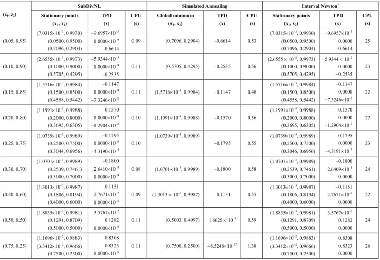
In Table 1 the results of phase stability tests for the citric acid (1) + butan-2-ol (2) binary system at 25ºC and different overall compositions are presented. The binary parameters of the NRTL model were taken from Gecegormez and Demirel (2005), which were presented by Lintomen et al. (2001). One can see in Table 1 that, for this system, solutions obtained in this work are in perfect agreement with the roots found by Gecegormez and Demirel (2005), which used an interval analysis algorithm. It can also be observed that the SubDivNL algorithm had lower computational effort in terms of CPU time that the SA algorithm (our results) and was shown to be much less time-consuming than the Interval Newton (IN/GB) algorithm reported on Gecegormez and Demirel (2005).

Table 1: Results of phase stability analysis for the citric acid (1) + butan-2-ol (2) system at 25ºC.

SubDivNL Simulated Annealing Interval Newton*

(z1, z2) Stationary points (x1, x2)

TPD (x)

CPU (s)

Global minimum (x1, x2)

TPD (x)

CPU (s)

Stationary points (x1, x2)

TPD (x)

CPU (s)

(0.05, 0.95)

(7.0315×10–3_{, 0.9930)}

(0.0500, 0.9500) (0.7096, 0.2904)

–9.6957×10–3

1.0000×10–9

–0.6614

0.09 (0.7096, 0.2904) –0.6614 0.53

(7.0315×10−3_{, 0.9930)}

(0.0500, 0.9500) (0.7096, 0.2904)

−9.6957×10–3

0.0000 –0.6614

25

(0.10, 0.90)

(2.6555×10–3_{, 0.9973)}

(0.1000, 0.9000) (0.5705, 0.4295)

–5.9344×10–3

1.0000×10–9

–0.2535

0.11 (0.5705, 0.4295) –0.2535 0.56

(2.6555 × 10−3_{, 0.9973)}

(0.1000, 0.9000) (0.5705, 0.4295)

−5.9344 × 10–2

0.0000 −0.2535

23

(0.15, 0.85)

(1.5716×10–3_{, 0.9984)}

(0.1500, 0.8500) (0.4558, 0.5442)

–0.1147 1.0000×10–9

–7.3246×10–2

0.11 (1.5716×10–3_{, 0.9984)} _{–0.1147 0.48}

(1.5716×10−3_{, 0.9984)}

(0.1500, 0.8500) (0.4558, 0.5442)

−0.1147 0.0000 −7.3246×10–2

22

(0.20, 0.80)

(1.1991×10–3_{, 0.9988)}

(0.2000, 0.8000) (0.3695, 0.6305)

–0.1570 1.0000×10–9

–1.2904×10–2

0.10 (1.1991×10–3_{, 0.9988)} _{–0.1570 0.56}

(1.1991×10−3_{, 0.9988)}

(0.2000, 0.8000) (0.3695, 0.6305)

–0.1570 0.0000 −1.2904×10–2

22

(0.25, 0.75)

(1.0739×10–3_{, 0.9989)}

(0.2500, 0.7500) (0.3044, 0.6956)

–0.1795 1.0000×10–9

–4.3190×10–4

0.10

(1.0739×10–3_{, 0.9989)}

–0.1795 0.55

(1.0739×10−3_{, 0.9989)}

(0.2500, 0.7500) (0.3046, 0.6956)

–0.1795 0.0000 −4.3191×10–4

23

(0.30, 0.70)

(1.0701×10–3_{, 0.9989)}

(0.2539, 0.7461) (0.3000, 0.7000)

–0.1800 2.6410×10–4

1.0000×10–9

0.08 (1.0701×10–3_{, 0.9989)} _{–0.1800 0.58}

(1.0701×10−3_{, 0.9989)}

(0.2539, 0.7461) (0.3000, 0.7000)

–0.1800 2.6409×10–4

0.0000 24

(0.40, 0.60)

(1.3013×10–3_{, 0.9987)}

(0.1806, 0.8194) (0.4000, 0.6000)

–0.1151 2.7671×10–2

1.0000×10–8

0.09 (1.3013 × 10–3_{, 0.9987)} _{–0.1151 0.55}

(1.3013×10−3_{, 0.9987)}

(0.1806, 0.8194) (0.4000, 0.6000)

–0.1151 2.7671×10–2

0.0000 22

(0.50, 0.50)

(1.8835×10–3_{, 0.9981)}

(0.1291, 0.8709) (0.5000, 0.5000)

3.5767×10–2

0.1282 1.0000×10–8

0.11 (0.5003, 0.4997) 1.6625 × 10–7 _0.59

(1.8835×10−3_{, 0.9981)}

(0.1291, 0.8709) (0.5000, 0.5000)

3.5767×10–2

0.1282 0.0000

24

(0.75, 0.25)

(1.1696×10–2_{, 0.9883)}

(3.3412×10–2_{, 0.9666)}

(0.7500, 0.2500)

0.8308 0.8323 1.0000×10–8

0.11 (0.7500, 0.2500) –8.5248×10–17 _1.38

(1.1696×10−2_{, 0.9883)}

(3.3412×10−2_{, 0.9666)}

(0.7500, 0.2500)

0.8308 0.8323 0.0000

26 *

(5)

Case 2: n-pentanol (1) + 2,2-dimethylbutane (2) system

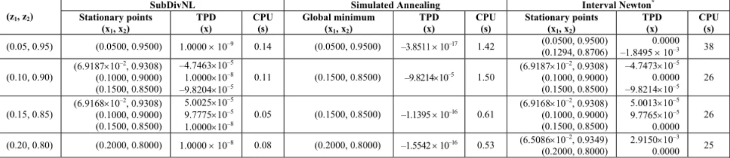
Results of phase stability analysis obtained in this work for the n-pentanol (1) + 2,2-dimethylbutane (2) system at 25 ºC and several global compositions are presented in Table 2. Results from the SA and SubDivNL algorithms are compared with solutions reported by Gecegormez and Demirel (2005). The NRTL parameters, which refer to a VLE set of parameters previously reported in the literature, were taken from Demirel and Gecegormez (1991).

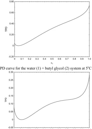
It can be observed in Table 2 that for the two overall compositions, z = (0.05, 0.95) and z = (0.20, 0.80), results obtained in this work are different from those presented by Gecegormez and Demirel (2005). The TPD curves for mixtures containing respectively 0.05 and 0.20 in mole fraction of n-pentanol are represented in Figures 1 and 2. As clearly shown in these figures, the nontrivial solutions reported by Gecegormez and Demirel (2005) are not true solutions for the phase stability test, so the system

has only one phase in both cases.

Moreover, the solutions presented in the literature are not stationary points on the TPD surface. In fact, the Euclidean norms of the set of equations calculated for such roots are far from zero: for z = (0.05, 0.95) and x = (0.1294, 0.8706), the value

found is

i _{i j}

TPD

x _≠

∂ ₌

∂ 0.0229, and for z = (0.20, 0.80)

and x = (6.5086 × 10-2, 0.9349), the result is 0.0292. For all overall compositions tested for this system, our calculations only indicated the existence of a one-phase, homogeneous system, which just corroborates phase equilibrium data reported by Sayegh and Ratcliff (1976).

Nevertheless, one should call attention to the fact that the use of a set of parameters coming from VLE to LLE calculations is not recommended (Poling et al., 2000). In this work, however, a parameter set from VLE (Demirel and Gecegormez, 1991) for LLE computations is applied just to enable numerical comparison with the results of Gecegormez and Demirel (2005).

Table 2: Results of phase stability analysis for the n-pentanol (1) + 2.2-dimetilbutane (2) system at 25ºC.

(z1, z2) Stationary points

(x1, x2)

TPD (x)

CPU (s)

TPD (x)

CPU (s)

TPD (x)

CPU (s)

(0.05, 0.95) (0.0500, 0.9500) 1.0000 × 10–9 _{0.14 (0.0500,}_0.9500)_–3.8511_×₁₀–17 _1.42 (0.0500, 0.9500)

(0.1294, 0.8706)

0.0000 –1.8495 × 10–3 38

(0.10, 0.90)

(6.9187×10–2_{, 0.9308)}

(0.1000, 0.9000) (0.1500, 0.8500)

–4.7463×10–5

1.0000×10–8

–9.8204×10–5

0.11 (0.1500, 0.8500) –9.8214×10–5 _1.50

(6.9187×10–2_{, 0.9308)}

(0.1000, 0.9000) (0.1500, 0.8500)

–4.7473×10–5

0.0000 –9.8214×10–5

26 (0.15, 0.85)

(6.9168×10–2_{, 0.9308)}

(0.1000, 0.9000) (0.1500, 0.8500)

5.0025×10–5

9.7775×10–5

1.0000×10–8

0.05 (0.1500, 0.8500) –1.1395 × 10–16 _0.61

(6.9168×10–2_{, 0.9308)}

(0.1000, 0.9000) (0.1500, 0.8500)

5.0013×10–5

9.7765×10–5

0.0000 26 (0.20, 0.80) (0.2000, 0.8000) 1.0000 × 10–8 _{0.08 (0.2000,}_0.8000)_–1.5542_×₁₀–16 _0.53 (6.5086×10–2, 0.9349)

(0.2000, 0.8000)

2.9150×10–3

0.0000 25 *

Results obtained from Gecegormez and Demirel (2005)

0 0.02 0.04 0.06 0.08 0.10 0.12 0.14 0.16 0.18 0.20

x1

-0.002 0 0.002 0.004 0.006 0.008 0.010 0.012 0.014 0.016 0.018 0.020

TP

D

(6)

0.02 0.06 0.10 0.14 0.18 0.22 0.26 0.30

x₁

-0.002 0 0.002 0.004 0.006 0.008 0.010

TP

D

Figure 2: TPD curve for the n-pentanol (1) + 2,2-dimetilbutane (2) system at 25 oC and z1 = 0.20.

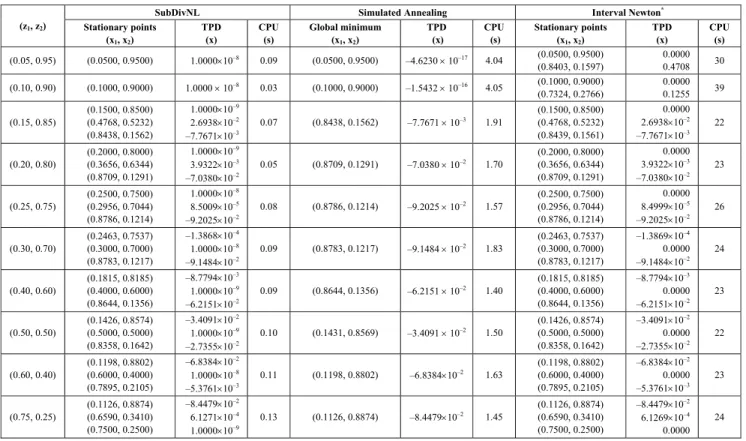
Case 3: water (1) + butyl glycol (2) system

The NRTL parameters for this system, which are presented in the literature (Demirel and Gecegormez, 1991) and refer to a set of parameters from VLE, were taken from Gecegormez and Demirel (2005). Solutions of the phase stability test in relation to LLE for the water (1) + butyl glycol (2) system at

5ºC and several global compositions are presented in Table 3. As depicted in Figures 3 and 4 the nontrivial roots reported by Gecegormez and Demirel (2005) for the water overall molar fractions of 0.05 and 0.10, respectively, are not true roots. According to the results from the SA and SubDivNL algorithms presented in this work, this system has only one stable phase at these compositions.

Table 3: Results of phase stability analysis for the water (1) + butyl glycol (2) system at 5ºC.

(z1, z2) Stationary points

(x1, x2)

TPD (x)

CPU (s)

TPD (x)

CPU (s)

TPD (x)

CPU (s)

(0.05, 0.95) (0.0500, 0.9500) 1.0000×10–8 _{0.09 (0.0500,}_0.9500)_–4.6230_×₁₀–17 _4.04 (0.0500, 0.9500)

(0.8403, 0.1597)

0.0000 0.4708 30 (0.10, 0.90) (0.1000, 0.9000) 1.0000 × 10–8 _{0.03 (0.1000,}_0.9000)_–1.5432_×₁₀–16 _4.05 (0.1000, 0.9000)

(0.7324, 0.2766)

0.0000 0.1255 39 (0.15, 0.85)

(0.1500, 0.8500) (0.4768, 0.5232) (0.8438, 0.1562)

1.0000×10–9

2.6938×10–2

–7.7671×10–3

0.07 (0.8438, 0.1562) –7.7671 × 10–3 _1.91

(0.1500, 0.8500) (0.4768, 0.5232) (0.8439, 0.1561)

0.0000 2.6938×10–2

–7.7671×10–3

22

(0.20, 0.80)

(0.2000, 0.8000) (0.3656, 0.6344) (0.8709, 0.1291)

1.0000×10–9

3.9322×10–3

–7.0380×10–2

0.05 (0.8709, 0.1291) –7.0380 × 10–2 _1.70

(0.2000, 0.8000) (0.3656, 0.6344) (0.8709, 0.1291)

0.0000 3.9322×10–3

–7.0380×10–2

23

(0.25, 0.75)

(0.2500, 0.7500) (0.2956, 0.7044) (0.8786, 0.1214)

1.0000×10–8

8.5009×10–5

–9.2025×10–2

0.08 (0.8786, 0.1214) –9.2025 × 10–2 _1.57

(0.2500, 0.7500) (0.2956, 0.7044) (0.8786, 0.1214)

0.0000 8.4999×10–5

–9.2025×10–2

26

(0.30, 0.70)

(0.2463, 0.7537) (0.3000, 0.7000) (0.8783, 0.1217)

–1.3868×10–4

1.0000×10–8

–9.1484×10–2

0.09 (0.8783, 0.1217) –9.1484 × 10–2 _1.83

(0.2463, 0.7537) (0.3000, 0.7000) (0.8783, 0.1217)

–1.3869×10–4

0.0000 –9.1484×10–2

24

(0.40, 0.60)

(0.1815, 0.8185) (0.4000, 0.6000) (0.8644, 0.1356)

–8.7794×10–3

1.0000×10–9

–6.2151×10–2

0.09 (0.8644, 0.1356) –6.2151 × 10–2 _1.40

(0.1815, 0.8185) (0.4000, 0.6000) (0.8644, 0.1356)

–8.7794×10–3

0.0000 –6.2151×10–2

23

(0.50, 0.50)

(0.1426, 0.8574) (0.5000, 0.5000) (0.8358, 0.1642)

–3.4091×10–2

1.0000×10–9

–2.7355×10–2

0.10 (0.1431, 0.8569) –3.4091 × 10–2 _1.50

(0.1426, 0.8574) (0.5000, 0.5000) (0.8358, 0.1642)

–3.4091×10–2

0.0000 –2.7355×10–2

22

(0.60, 0.40)

(0.1198, 0.8802) (0.6000, 0.4000) (0.7895, 0.2105)

–6.8384×10–2

1.0000×10–8

–5.3761×10–3

0.11 (0.1198, 0.8802) –6.8384×10–2 _1.63

(0.1198, 0.8802) (0.6000, 0.4000) (0.7895, 0.2105)

–6.8384×10–2

0.0000 –5.3761×10–3

23

(0.75, 0.25)

(0.1126, 0.8874) (0.6590, 0.3410) (0.7500, 0.2500)

–8.4479×10–2

6.1271×10–4

1.0000×10–9

0.13 (0.1126, 0.8874) –8.4479×10–2 _1.45

(0.1126, 0.8874) (0.6590, 0.3410) (0.7500, 0.2500)

–8.4479×10–2

6.1269×10–4

0.0000 24 *

(7)

0 0.1 0.2 0.3 0.4 0.5 0.6 0.7 0.8 0.9 1.0

x₁

-0.20 0 0.20 0.40 0.60 0.80

TP

D

Figure 3: TPD curve for the water (1) + butyl glycol (2) system at 5oC and z1 = 0.05.

0 0.1 0.2 0.3 0.4 0.5 0.6 0.7 0.8 0.9 1.0 x1

-0.05 0 0.05 0.10 0.15 0.20 0.25 0.30

TP

D

Figure 4: TPD curve for the water (1) + butyl glycol (2) system at 5oC and z1 = 0.10.

Case 4: water (1) + citric acid (2)+ 2-butanol (3) system

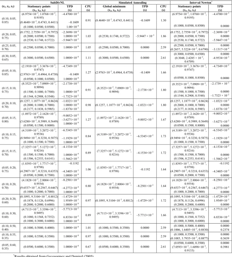
The LLE binary parameters of the NRTL model for this system were used as presented by Gecegormez and Demirel (2005), originally reported by Lintomen et al. (2001). Table 4 contains the results of phase stability analysis for this ternary system at 25ºC and different overall compositions. Solutions found in this work are compared with the roots presented by Gecegormez and Demirel (2005).

As shown in Table 4, some divergences between our results and those presented in the literature can be verified. For the global composition of z = (0.10, 0.05, 0.85), the composition with the lowest TPD value found in this work was x = (8.4640×10-2, 0.4743, 0.4411) with TPD = -0.1609, while this root is not reported in the literature. Also, for the global composition z = (0.05, 0.10, 0.85) the SubDivNL and SA algorithms found an unstable composition, not reported in the literature. It can also be verified

from Table 4 that for the last third overall composition, a second root, found in the literature, was not found by the SA and SubDivNL algorithms.

Another discrepancy was verified for the two overall compositions: a) z = (0.25, 0.05, 0.70) and b)

z = (0.30, 0.05, 0.65) that correspond to mass fractions of a) z = (0.0682, 0.1456, 0.7862) and b) z

(8)

Table 4: Results of phase stability analysis for the water (1) + citric acid (2) + 2-butanol (3) system at 45ºC.

SubDivNL Simulated Annealing Interval Newton*

(z1, z2, z3) Stationary points

(x1, x2, x3)

TPD (x)

CPU (s)

Global minimum (x1, x2, x3)

TPD (x)

CPU (s)

Stationary points (x1, x2, x3)

TPD (x)

(6.9754×10−2_{, 1.0768×10}−2_,

0.9195)

–4.4700×10–3

(8.4640×10−2_{, 0.4743, 0.4411)} _–0.1609

(0.10, 0.05, 0.85)

(0.1000, 0.0500, 0.8500) 1.00×10–8

0.91 (8.4640×10−2_{, 0.4743, 0.4411)} _–0.1609 _1.30

(6.9754×10−2_{, 1.0768×10}−2_,

0.9195) (0.1000, 0.0500, 0.8500)

–4.4700×10–3

0.0000 (0.20, 0.05,

0.75)

(0.1752, 2.7558×10−2_{, 0.7972)}

(0.2000, 0.0500, 0.7500) (0.2530, 0.1748, 0.5722)

–2.3698×10–4

1.0000×10–8

–5.9447×10–3

1.03 (0.2530, 0.1748, 0.5722) –5.9447 × 10–3_1.86

(0.1752, 2.7558×10−2_{, 0.7972)}

(0.2000, 0.0500, 0.7500) (0.2530, 0.1748, 0.5722)

–2.3698×10–4

0.0000 –5.9447×10–3

(0.25, 0.05,

0.70) (0.2500, 0.0500, 0.7000) 1.0000×10

–8 _1.05 _{(0.2500, 0.0500, 0.7000)} _0.0000 _2.59 (0.2500, 0.0500, 0.7000)

(0.2657, 5.5224×10−2_{, 0.6790)}

0.0000 –3.1317×10–4

(0.30, 0.05,

0.65) (0.3000, 0.0500, 0.6500) 1.0000×10

–8 _1.11 _{(0.3000, 0.0500, 0.6500)} _0.0000 _2.61

(0.3000, 0.0500, 0.6500) (0.3048, 2.4285 × 10−2_,

0.6709)

0.0000 -4.9534×10–3

(2.1910×10−2_{, 3.3676×10}−3_,

0.9747)

–4.7349×10–2

(2.9763×10−2_{, 0.4964, 0.4738)} _–0.1409

(0.05, 0.10, 0.85)

(0.0500, 0.1000, 0.8500) 1.0000×10–8

1.27 (2.9763×10−2_{, 0.4964, 0.4738)} _–0.1409 _1.66

(2.1910×10−2_{, 3.3676×10}−3_,

0.9747) (0.0500, 0.1000, 0.8500)

–4.7349×10–2

0.0000 (8.3523×10−2_{, 7.0909×10}−3_,

0.9094)

–2.1738×10–2

(0.1500, 0.1000, 0.7500) 1.0000×10–9

(0.15, 0.10, 0.75)

(0.1544, 0.2908, 0.5548) –1.7323×10–2

0.91 (8.3523×10

−2_{, 7.0909×10}−3_,

0.9094) –2.1738×10

–2_1.80

(8.3523×10−2_{, 7.0909×10}−3_,

0.9094) (0.1500, 0.1000, 0.7500) (0.1544, 0.2908, 0.5548)

–2.1739 × 10–2

0.0000 –1.7323 × 10–2

(0.20, 0.10, 0.70)

(0.1257, 1.1877×10−2_{, 0.8624)}

(0.2000, 0.1000, 0.7000) (0.2177, 0.1838, 0.5985)

–1.0321×10–2

1.0000×10–9

–1.8376×10–3

0.98 (0.1257, 1.1877×10−2_{, 0.8624)} _{–1.0321×10}–2_1.80

(0.1257, 1.1877×10−2_{, 0.8624)}

(0.2000, 0.1000, 0.7000) (0.2177, 0.1838, 0.5985)

–1.0321×10–2

0.0000 –1.8376×10–3

(0.05, 0.15, 0.80)

(1.8972×10−2_{, 2.1628×10}−3_,

0.9789) (3.6280×10−2_{, 0.3989, 0.5649)}

(0.0500, 0.1500, 0.8000)

–9.0052×10–2

–3.6271×10–2

1.0000×10–9

1.27 (1.8972×10

−2_{, 2.1628×10}−3_,

0.9789) –9.0052×10

–2_1.67

(1.8972×10−2_{, 2.1628×10}−3_,

0.9789) (3.6280×10−2_{, 0.3989, 0.5649)}

(0.0500, 0.1500, 0.8000)

–9.0052×10–2

–3.6271×10–2

0.0000 (0.10, 0.15,

0.75)

(4.3189×10−2_{, 3.2072×10}−3_,

0.9536) (8.9494×10−2_{, 0.3230, 0.5875)}

(0.1000, 0.1500, 0.7500)

–6.5345×10–2

–1.1929×10–2

1.0000×10–9

0.84 (4.3189×10

−2_{, 3.2072×10}−3_,

0.9536) –6.5345×10

–2_1.73

(4.3189×10−2_{, 3.2072×10}−3_,

0.9536) (8.9494×10−2_{, 0.3230, 0.5875)}

(0.1000, 0.1500, 0.7500)

–6.5345×10–2

–1.1929×10–2

0.0000 (0.15, 0.15,

0.70)

(7.3257×10−2_{, 5.1272×10}−3_,

0.9216) (0.1500, 0.1500, 0.7000) (0.1506, 0.2353, 0.6141)

–4.1534×10–2

1.0000×10–9

–1.5662×10–3

0.89 (7.3257×10

−2_{, 5.1272×10}−3_,

0.9216) –4.1534×10

–2_1.72

(7.3257×10−2_{, 5.1272×10}−3_,

0.9216) (0.1500, 0.1500, 0.7000) (0.1506, 0.2353, 0.6141)

–4.1534×10–2

0.0000 –1.5662×10–3

(0.05, 0.20, 0.75)

(1.8393×10−2_{, 1.7717×10}−3_,

0.9798) (4.2907×10−2_{, 0.3218, 0.6353)}

(0.0500, 0.2000, 0.7500)

–0.1192 –4.3405×10–3

1.0000×10–8

1.06 (1.8393×10

−2_{, 1.7717×10}−3_,

0.9798) –0.1192 1.64

(1.8393×10−2_{, 1.7717×10}−3_,

0.9798) (4.2907×10−2_{, 0.3218, 0.6353)}

(0.0500, 0.2000, 0.7500)

–0.1192 –4.3405×10–3

0.0000 (0.10, 0.20,

0.70)

(4.1828×10−2_{, 2.8004×10}−3_,

0.9554) (9.6537×10−2_{, 0.2567, 0.6467)}

(0.1000, 0.2000, 0.7000)

–8.2501×10–2

–4.2772×10–4

1.0000×10–8

0.80 (4.1828×10

−2_{, 2.8004×10}−3_,

0.9554) –8.2501×10

–2_1.64

(4.1828×10−2_{, 2.8004×10}−3_,

0.9554) (9.6537×10−2_{, 0.2567, 0.6467)}

(0.1000, 0.2000, 0.7000)

–8.2501×10–2

–4.2773×10–4

0.0000 (0.20, 0.20,

0.60)

(0.1095, 9.3104×10−3_{, 0.8812)}

(0.1878, 0.1126, 0.6996) (0.2000, 0.2000, 0.6000)

–1.4729×10–2

1.9549×10–3

1.0000×10–8

0.97 (0.1095, 9.3104×10−3_{, 0.8812)} _{–1.4729×10}–2_1.72

(0.1095, 9.3104×10−3_{, 0.8812)}

(0.1878, 0.1126, 0.6996) (0.2000, 0.2000, 0.6000)

–1.4729×10–2

1.9549×10–3

0.0000 (0.10, 0.30,

0.60)

(4.7113×10−2_{, 3.3396×10}−3_,

0.9495) (0.1080, 0.1568, 0.7352) (0.1000, 0.3000, 0.6000)

–5.7713×10–2

6.8336×10–3

1.0000×10–8

0.89 (4.7113×10

−2_{, 3.3396×10}−3_,

0.9495) –5.7713×10

–2_1.66

(4.7113×10−2_{, 3.3396×10}−3_,

0.9495) (0.1080, 0.1568, 0.7352) (0.1000, 0.3000, 0.6000)

–5.7713×10–2

6.8336×10–3

0.0000 (0.10, 0.50,

0.40) (0.1000, 0.5000, 0.4000) 1.0000×10

–8 _1.01 _{(0.1000, 0.5500, 0.3500)} _0.0000 _2.59 (0.1000, 0.5000, 0.4000)

(0.1006, 1.6405×10−2_{, 0.8830)}

0.0000 0.2374 (0.10, 0.55,

0.35) (0.1000, 0.5500, 0.3500) 1.0000×10

–8 _0.97 _{(0.1000, 0.5500, 0.3500)} _0.0000 _2.59 (0.1000, 0.5500, 0.3500)

(0.1085, 3.7935×10−3_{, 0.8877)}

0.0000 0.3639 (0.05, 0.60,

0.35) (0.0500, 0.6000, 0.3500) 1.0000×10

–8 _0.67 _{(0.0500, 0.6000, 0.3500)} _0.0000 _2.61

(0.0500, 0.6000, 0.3500) (7.0593×10−2_{, 1.6098×10}−2_,

0.9133)

0.0000 0.3981 *

(9)

0.1 0.2 0.3 0.4 0.5 0.6 0.7 0.8 0.9

w3 0.00

0.02 0.04 0.06 0.08 0.10 0.12 0.14 0.16 0.18

w2

(a) (b)

Figure 5: Experimental diagram of the water (1) + citric acid (2) + 2-butanol (3) ternary system at 25 oC.

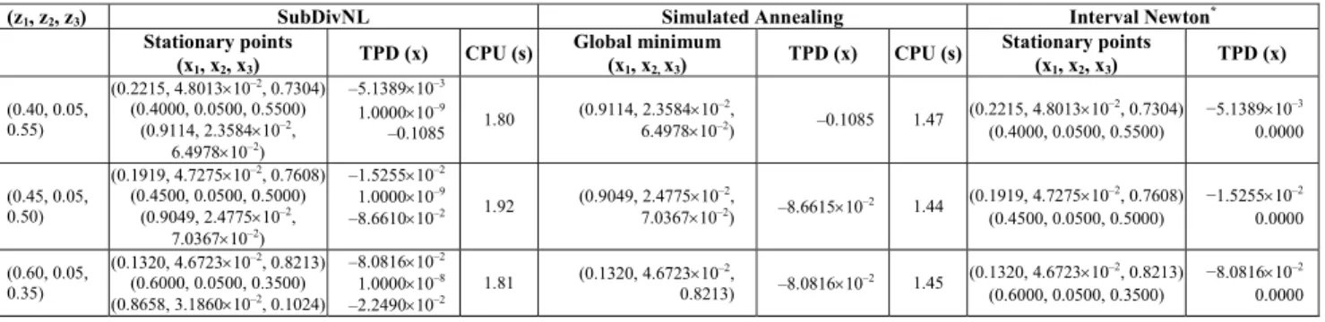
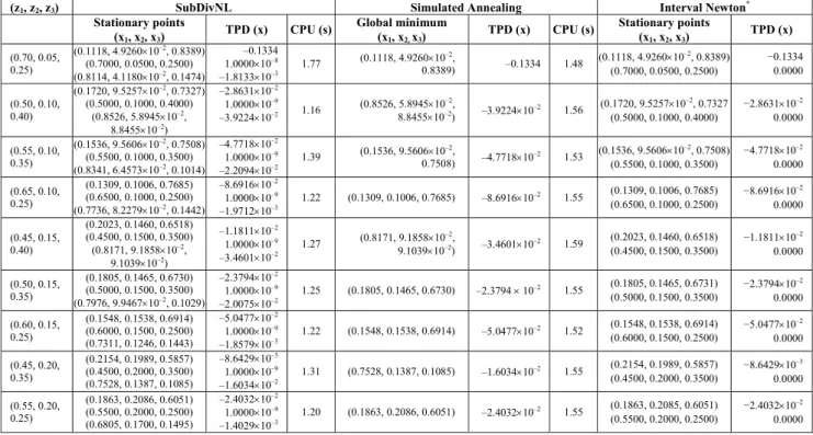
Case 5: acetonitrile (1) + benzene (2) + n-heptane (3) system

Table 5 contains the results of phase stability analysis for this ternary system at 45ºC and different overall compositions. Solutions found in this work are compared with the roots presented by Gecegormez and Demirel (2005). As shown in this table, application of the subdivision algorithm indicated the existence of a third root for all compositions analyzed. This additional root however is not presented in the work of Gecegormez and Demirel (2005). For this problem, the Simulated Annealing algorithm had a better performance in terms of CPU time than the subdivision method.

Case 6: n-propanol (1) + n-butanol (2) + benzene (3) + water (4) system

Solutions of the phase stability test for this system are presented in Table 6. The binary interaction parameters for the NRTL model were taken from Tessier et al. (2000). Aiming at reducing

the computational effort, the maximum number of subdivisions was set to four. It can be verified that both algorithms employed in this work were able to find the same solutions as those presented in the literature (Tessier et al., 2000). The CPU time values listed in this table confirm the advantageous performance of the Simulated Annealing algorithm for systems with larger number of components.

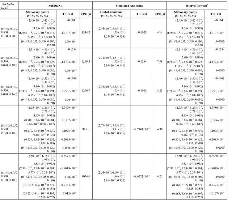
Case 7: n-propanol (1) + n-butanol (2) + benzene (3) + ethanol (4) + water (5) system

Table 7 depicts the results of the thermodynamic stability test for this multicomponent system. For this system the NRTL parameters were also taken from Tessier et al. (2000), whose results are compared in this work. The maximum number of subdivisions was again set to four. Although the Simulated Annealing algorithm had a better performance in terms of CPU time than the SubDivNL, solutions obtained with both mathematical methods employed in this work are in agreement with those reported by Tessier et al. (2000), who used the Interval Newton method.

Table 5: Results of phase stability analysis for the acetonitrile (1) + benzene (2) + n-heptane (3) system at 45ºC.

(z1, z2, z3) SubDivNL Simulated Annealing Interval Newton*

TPD (x) CPU (s) Global minimum (x1, x2, x3)

TPD (x) CPU (s) Stationary points (x1, x2, x3)

TPD (x)

(0.40, 0.05, 0.55)

(0.2215, 4.8013×10–2_{, 0.7304)}

(0.4000, 0.0500, 0.5500) (0.9114, 2.3584×10–2_,

6.4978×10–2₎

–5.1389×10–3

1.0000×10–9

–0.1085 1.80

(0.9114, 2.3584×10–2_,

6.4978×10–2₎ –0.1085 1.47

(0.2215, 4.8013×10–2_{, 0.7304)}

(0.4000, 0.0500, 0.5500)

−5.1389×10–3

0.0000 (0.45, 0.05,

0.50)

(0.1919, 4.7275×10–2_{, 0.7608)}

(0.4500, 0.0500, 0.5000) (0.9049, 2.4775×10–2_,

7.0367×10–2₎

–1.5255×10–2

1.0000×10–9

–8.6610×10–2 1.92

(0.9049, 2.4775×10–2_,

7.0367×10–2₎ –8.6615×10–2 1.44

(0.1919, 4.7275×10–2_{, 0.7608)}

(0.4500, 0.0500, 0.5000)

−1.5255×10–2

0.0000 (0.60, 0.05,

0.35)

(0.1320, 4.6723×10–2_{, 0.8213)}

(0.6000, 0.0500, 0.3500) (0.8658, 3.1860×10–2_{, 0.1024)}

–8.0816×10–2

1.0000×10–8

–2.2490×10–2

1.81 (0.1320, 4.6723×10

–2_,

0.8213) –8.0816×10

–2 _1.45 (0.1320, 4.6723×10–2, 0.8213)

(0.6000, 0.0500, 0.3500)

−8.0816×10–2

(10)

Continuation Table 5

(z1, z2, z3) SubDivNL Simulated Annealing Interval Newton*

TPD (x) CPU (s) Global minimum (x1, x2, x3)

TPD (x) CPU (s) Stationary points (x1, x2, x3)

TPD (x)

(0.70, 0.05, 0.25)

(0.1118, 4.9260×10–2_{, 0.8389)}

(0.7000, 0.0500, 0.2500) (0.8114, 4.1180×10–2_{, 0.1474)}

–0.1334 1.0000×10–8

–1.8133×10–3

1.77 (0.1118, 4.9260×10

–2_,

0.8389) –0.1334 1.48

(0.1118, 4.9260×10–2_{, 0.8389)}

(0.7000, 0.0500, 0.2500)

−0.1334 0.0000 (0.50, 0.10,

0.40)

(0.1720, 9.5257×10–2_{, 0.7327)}

(0.5000, 0.1000, 0.4000) (0.8526, 5.8945×10–2_,

8.8455×10–2₎

–2.8631×10–2

1.0000×10–9

–3.9224×10–2 1.16

(0.8526, 5.8945×10–2_,

8.8455×10–2₎ –3.9224×10–2 1.56

(0.1720, 9.5257×10–2_{, 0.7327}

(0.5000, 0.1000, 0.4000)

−2.8631×10–2

0.0000 (0.55, 0.10,

0.35)

(0.1536, 9.5606×10–2_{, 0.7508)}

(0.5500, 0.1000, 0.3500) (0.8341, 6.4573×10–2_{, 0.1014)}

–4.7718×10–2

1.0000×10–9

–2.2094×10–2

1.39 (0.1536, 9.5606×10

–2_,

0.7508) –4.7718×10

–2 _1.53 (0.1536, 9.5606×10 –2_{, 0.7508)}

(0.5500, 0.1000, 0.3500)

−4.7718×10–2

0.0000 (0.65, 0.10,

0.25)

(0.1309, 0.1006, 0.7685) (0.6500, 0.1000, 0.2500) (0.7736, 8.2279×10–2_{, 0.1442)}

–8.6916×10–2

1.0000×10–9

–1.9712×10–3

1.22 (0.1309, 0.1006, 0.7685) –8.6916×10–2 _1.55 (0.1309, 0.1006, 0.7685)

(0.6500, 0.1000, 0.2500)

−8.6916×10–2

0.0000 (0.45, 0.15,

0.40)

(0.2023, 0.1460, 0.6518) (0.4500, 0.1500, 0.3500) (0.8171, 9.1858×10–2_,

9.1039×10–2₎

–1.1811×10–2

1.0000×10–9

–3.4601×10–2

1.27 (0.8171, 9.1858×10

–2_,

9.1039×10–2₎ –3.4601×10–2 1.59

(0.2023, 0.1460, 0.6518) (0.4500, 0.1500, 0.3500)

−1.1811×10–2

0.0000 (0.50, 0.15,

0.35)

(0.1805, 0.1465, 0.6730) (0.5000, 0.1500, 0.3500) (0.7976, 9.9467×10–2_{, 0.1029)}

–2.3794×10–2

1.0000×10–9

–2.0075×10–2

1.25 (0.1805, 0.1465, 0.6730) –2.3794 × 10–2 _1.55 (0.1805, 0.1465, 0.6731)

(0.5000, 0.1500, 0.3500)

−2.3794×10–2

0.0000 (0.60, 0.15,

0.25)

(0.1548, 0.1538, 0.6914) (0.6000, 0.1500, 0.2500) (0.7311, 0.1246, 0.1443)

–5.0477×10–2

1.0000×10–9

–1.8579×10–3

1.22 (0.1548, 0.1538, 0.6914) –5.0477×10–2 _1.52 (0.1548, 0.1538, 0.6914)

(0.6000, 0.1500, 0.2500)

−5.0477×10–2

0.0000 (0.45, 0.20,

0.35)

(0.2154, 0.1989, 0.5857) (0.4500, 0.2000, 0.3500) (0.7528, 0.1387, 0.1085)

–8.6429×10–3

1.0000×10–9

–1.6034×10–2

1.31 (0.7528, 0.1387, 0.1085) –1.6034×10–2 _1.55 (0.2154, 0.1989, 0.5857)

(0.4500, 0.2000, 0.3500)

−8.6429×10–3

0.0000 (0.55, 0.20,

0.25)

(0.1863, 0.2086, 0.6051) (0.5500, 0.2000, 0.2500) (0.6805, 0.1700, 0.1495)

–2.4032×10–2

1.0000×10–9

–1.4029×10–3

1.20 (0.1863, 0.2086, 0.6051) –2.4032×10–2 _1.55 (0.1863, 0.2085, 0.6051)

(0.5500, 0.2000, 0.2500)

−2.4032×10–2

0.0000

*

Results obtained from Gecegormez and Demirel (2005)

Table 6: Results of phase stability analysis for the n-propanol (1) + n-butanol (2) + benzene (3) + water(4) system.

(z1, z2, z3, z4) Stationary points

(x1, x2, x3, x4, x5)

TPD (x) CPU (s) Global minimum (x1, x2, x3, x4)

TPD (x) CPU (s) Stationary points (x1, x2, x3, x4)

TPD (x)

(1.81×10–2_{, 6.20}_×₁₀–4_,

4.48×10–3_{, 0.977)}

–0.3398 (1.81×10–2_{, 6.20}_×₁₀–4_,

4.48×10–3_{, 0.977)}

–0.3398 (4.61×10–2_{, 1.89}_×₁₀–2_,

0.916, 1.87×10–2₎

–3.3651×10–2_(4.61_×₁₀–2_{, 1.89}_×₁₀–2_,

0.916, 1.87×10–2₎

–3.3650×10–2

(0.148, 0.052, 0.600, 0.200)

(0.148, 0.052, 0.600, 0.200) 1.0000×10–9

292.8 (1.81×10

–2_{, 6.20}_×₁₀–4_,

4.48×10–3_{, 0.977)} –0.3398 2.47

(0.148, 0.052, 0.600, 0.200) 0.0000 (2.41×10–2_{, 7.86}_×₁₀–4_,

4.74×10–3_{, 0.970)}

–0.3110 (2.41×10–2_{, 7.86}_×₁₀–4_,

4.74×10–3_{, 0.970)}

–0.3110 (8.20×10–2_{, 3.07}_×₁₀–2_,

0.854, 3.29×10–2₎

–3.1279×10–3_(8.20_×₁₀–2_{, 3.07}_×₁₀–2_,

0.854, 3.29×10–2₎

–3.1279×10–3

(0.148, 0.052, 0.700, 0.100)

(0.148, 0.052, 0.700, 0.1000)

1.0000×10–8

303.5 (2.41×10

–2_{, 7.86}_×₁₀–4_,

4.74×10–3_{, 0.970)} –0.3110 2.58

(0.148, 0.052, 0.700, 0.1000)

0.0000 (3.32×10–2_{, 2.69}_×₁₀–3_,

6.71×10–3_{, 0.957)}

–7.3626×10–2_(3.32_×₁₀–2_{, 2.69}_×₁₀–3_,

6.71×10–3_{, 0.957)}

–7.3630×10–2

(0.206, 9.47×10–2_{, 0.140,}

0.560)

1.0660×10–2_(0.206,_9.47_×₁₀–2_{, 0.140,}

0.560)

1.0660×10–2

(0.25, 0.15, 0.35, 0.25)

(0.250, 0.150, 0.350, 0.250)

1.0000 × 10–8

278.2 (3.32×10

–2_{, 2.69}_×₁₀–3_,

6.71×10–3_{, 0.957)} –7.3626×10–2 2.69

(0.250, 0.150, 0.350, 0.250)

0.0000 (3.67×10–2_{, 2.98}_×₁₀–3_,

7.37×10–3_{, 0.953)}

–3.8665×10–2_(3.67_×₁₀–2_{, 2.98}_×₁₀–3_,

7.37×10–3_{, 0.953)}

–3.8670×10–2

(0.195, 7.86×10–2_{, 0.114,}

0.613)

2.6680×10–2_(0.195,_7.86_×₁₀–2_{, 0.114,}

0.613)

2.2680×10–2

(0.25, 0.15, 0.40, 0.20)

(0.250, 0.150, 0.400, 0.200)

1.0000×10–8

269.6 (3.67 × 10

–2_{, 2.98}_×₁₀–3_,

7.37 × 10–3_{, 0.953)} –3.8666 × 10–2 2.75

(0.250, 0.150, 0.400, 0.200)

0.0000 (3.53×10–2_{, 5.73}_×₁₀–3_,

6.75×10–3_{, 0.952)}

3.0790×10–2 _(3.53_×₁₀–2_{, 5.73}_×₁₀–3_,

6.75×10–3_{, 0.952)}

3.0790×10–2

(0.133, 8.02×10–2_,

5.20×10–2_{, 0.735)}

6.5320×10–2 _{(0.133, 8.02}_×₁₀–2_,

5.20×10–2_{, 0.735)}

6.5320×10–2

(0.25, 0.25, 0.25, 0.25)

(0.250, 0.250, 0.250, 0.250)

1.0000×10–8

271.1 (0.250, 0.250, _{0.250, 0.250)} 1.0015 × 10–0 _5.19

(0.250, 0.250, 0.250, 0.250)

0.0000

*

(11)

Table 7: Results of phase stability analysis for the n-propanol (1) +

n-butanol (2) + benzene (3) + ethanol (4) + water (5) system.

(z1, z2, z3,

z4, z5)

Stationary points (x1, x2, x3, x4, x5)

TPD (x) CPU (s) Global minimum (x1, x2, x3, x4, x5)

TPD (x) CPU (s) Stationary points (x1, x2, x3, x4, x5)

TPD (x)

(2.43×10–2_{, 5.45}_×₁₀–4_,

1.73×10–3_,

3.55×10–2_{, 0.938)}

–0.1043 (2.43×10–2_{, 5.45}_×₁₀–4_,

1.73×10–3_,

3.55×10–2_{, 0.938)}

–0.1043

(6.98×10–2_{, 2.26}_×₁₀–2_{, 0.811,}

5.15×10–2_{, 4.52}_×₁₀–2₎

–4.2107×10–3_(6.98_×₁₀–2_{, 2.26}_×₁₀–2_{, 0.811,}

5.15×10–2_{, 4.52}_×₁₀–2₎

–4.2107×10–3

(0.148, 0.052, 0.500, 0.100, 0.200)

1.00×10–8

1314.2

(2.43×10–2_{, 5.45}_×₁₀–4_,

1.73×10–3_,

3.55×10–2_{, 0.938)}

–0.1043 4.14

(0.148, 0.052, 0.500, 0.100, 0.200)

0.0000 (2.31×10–2_{, 4.81}_×₁₀–4_,

1.42×10–3_,

2.89×10–2_{, 0.946)}

–0.1284 (2.31×10–2_{, 4.81}_×₁₀–4_,

1.42×10–3_,

2.89×10–2_{, 0.946)}

–0.1284

(6.90×10–2_{, 2.26}_×₁₀–2_{, 0.822,}

4.30×10–2_{, 4.32}_×₁₀–2₎

–4.4793×10–3 _(6.90_×₁₀–2_{, 2.62}_×₁₀–2_{, 0.822,}

4.30 × 10–2_{, 4.33}_×₁₀–2₎

–4.4793×10–3

(0.148, 0.052, 0.540, 0.080, 0.180)

1.00×10–8

1269.3

(2.31×10–2_{, 4.81}_×₁₀–4_,

1.42×10–3_,

2.89×10–2_{, 0.946)}

–0.1284 7.98

(0.148, 0.052, 0.540, 0.080, 0.180)

0.0000 (2.49×10–2_{, 5.52}_×₁₀–4_,

1.59×10–3_,

3.14×10–2_{, 0.942)}

–0.1086 (2.49×10–2_{, 5.52}_×₁₀–4_,

1.59×10–3_,

3.14×10–2_{, 0.942)}

–0.1068

(7.99×10–2_{, 2.68}_×₁₀–2_{, 0.794,}

4.85×10–2_{, 5.04}_×₁₀–2₎

–1.9581×10–3_(7.99_×₁₀–2_{, 2.68}_×₁₀–2_{, 0.794,}

4.85×10–2_{, 5.04}_×₁₀–2₎

–1.9581×10–3

(0.148, 0.052, 0.560, 0.080, 0.160)

1.00×10–8

1296.7

(2.45×10–2_{, 5.83}_×₁₀–4_,

1.63×10–3_,

3.13×10–2_{, 0.942)}

–0.1068 8.23

(0.148, 0.052, 0.560, 0.080, 0.160)

0.0000 (2.95×10–2_{, 8.25}_×₁₀–4_,

2.71×10–3_,

4.93×10–2_{, 0.918)}

–4.7479×10–2 _(2.95_×₁₀–2_{, 8.25}_×₁₀–4_,

2.71×10–3_,

4.93×10–2_{, 0.918)}

–4.7480×10–2

(0.108, 3.68×10–2_{, 0.684,}

8.60×10–2_{, 8.60}_×₁₀–2₎

1.0397×10–4_(0.108,_3.68_×₁₀–2_{, 0.684,}

8.60×10–2_{, 8.60}_×₁₀–2₎

1.0396×10–4

(0.119, 4.13×10–2_{, 0.639,}

9.46×10–2_{, 0.105)}

1.1076×10–4_(0.119,_4.13_×₁₀–2_{, 0.639,}

9.46×10–2_{, 0.105)}

1.1075×10–4

(0.136, 3.92×10–2_{, 0.152,}

0.156, 0.518)

6.2085×10–3_(0.136,_3.92_×₁₀–2_{, 0.152,}

0.156, 0.518)

6.2085×10–3

(0.148, 0.052, 0.500, 0.120, 0.180)

1.0000×10–8

915.0

(2.79×10–2_{, 8.95}_×₁₀–4_,

3.11×10–3_,

4.99×10–2_{, 0.918)}

–4.7402×10–2 _4.30

(0.148, 0.052, 0.500, 0.120, 0.180)

0.0000 (2.60×10–2_{, 6.18}_×₁₀–4_,

1.93×10–3_,

3.83×10–2_{, 0.933)}

–8.6575×10–2 _(2.60_×₁₀–2_{, 6.18}_×₁₀–4_,

1.93×10–3_,

3.83×10–2_{, 0.933)}

–8.6580×10–2

(7.96×10–2_{, 2.63}_×₁₀–2_{, 0.784.}

5.77×10–2_{, 5.24}_×₁₀–2₎

–1.9019×10–3_(7.96_×₁₀–2_{, 2.63}_×₁₀–2_{, 0.784,}

5.77×10–2_{, 5.24}_×₁₀–2₎

–1.9019×10–3

(0.148, 0.052, 0.520, 0.100, 0.180)

1.00×10–9 _{(0.148, 0.052, 0.520, 0.100,}

0.180)

0.0000 (0.162, 5.32 × 10–2_{, 0.271,}

0.128, 0.385)

8.2383×10–5 _{(0.162, 5.32}_×₁₀–2_{, 0.271,}

0.128, 0.385)

8.2373×10–5

(0.148, 0.052, 0.520, 0.100, 0.180)

(0.163, 5.64 × 10–2_{, 0.397,}

0.116, 0.267)

–1.012×10–4

1074.6

(2.55×10–2_{, 6.09}_×₁₀–4_,

1.86×10–3_,

3.81×10–2_{, 0.934)}

–8.6572×10–2 _4.25

(0.163, 5.64×10–2_{, 0.397,}

0.116, 0.267)

–1.0107×10–4 *

Results obtained from Tessier et al. (2000).

CONCLUSIONS

In this work thermodynamic phase stability with two stochastic global algorithms was examined for binary, ternary and multicomponent liquid mixtures using the NRTL activity coefficient model. Results of application of the subdivision algorithm to liquid-liquid equilibrium calculations show that it was able to find all roots of phase stability tests for the systems investigated with relatively short CPU times for binary and ternary systems. Simulated Annealing was shown to be reliable and robust for systems with

larger numbers of components. In a general sense, the two algorithms are relatively simple, provide reliable solutions for phase stability analysis, are easy to implement and require relatively low computational effort.

NOMENCLATURE

d problem dimension (-)

f(x) nonlinear equation (-)

(12)

equations

R multidimensional rectangle (-)

k

a lower coordinate of the “child” rectangles at “k” dimension

(-)

k

b upper coordinate of the “child” rectangles at “k” dimension

(-)

Ak lower coordinate of the

“parent” rectangles at “k” dimension

(-)

Bk upper coordinate of the

“parent” rectangles at “k” dimension

(-)

NRTL nonrandom two liquid (-)

i subdivision level (-)

y vector of random point in Rij

and vapor phase mole fraction

(-)

xij middle point of the rectangle “j” at the subdivision level “i”’

(-)

x vector of liquid phase mole fraction

(-)

z vector of global mole composition

(-)

T temperature (-)

T0 initial annealing temperature (-)

iRan sample number in Rij (-)

iMax maximum subdivision number

(-)

iCov maximum coverage number (-)

TPD tangent plane distance (-)

Greek Letters

k

ν

coordinate of the middle point of “parent” rectangle at “k” dimension

(-)

i

γ

activity coefficient of component “i”

(-)

ij

τ

subdivision parameter of the rectangle “j” at the

subdivision level “i”

(-)

αm,n matrix of zero and one

elements

(-)

Subscripts

0 pure component (-)

n number of components in the mixture and nth components of the system

(-)

ACKNOWLEDGEMENTS

The authors thank CENPES/PETROBRAS, FAPERGS and CNPq for the scholarships and financial support of this work.

REFERENCES

Baker, L. E., Pierce, A. C. and Luks, K. D., Soc. Pet. Eng. J., 22, 731 (1982).

Bonilla-Petriciolet, A., Vazquez-Roman, R., Iglesias-Silva, G. A. and Hall, K. R., Performance of stochastic global optimization in the calculation of phase stability analyses for nonreactive and reactive mixtures,Ind. Eng. Chem. Res., 45, 4764 (2006).

Carvalho Jr., R. N., Corazza, M. L., Cardozo-Filho, L. and Meireles, M. A. A., Phase equilibrium for (camphor+CO2), (camphor+propane), and (camphor +CO2+propane), J. Chem. Eng. Data, 51, 997 (2006).

Corazza, M. L., Corazza, F. C., Cardozo Filho, L. and Dariva, C., A subdivision algorithm for phase equilibrium calculations at high pressures, Braz. J. Chem. Eng, In press (2007).

Corazza, M. L., Filho, L. C., Oliveira, J. V. and Dariva, C., A robust strategy for SLV equilibrium calculations at high pressures, Fluid Phase Equilibria, 221, 113 (2004).

Demirel, Y. and Gecegormez, H., Simultaneous representation of excess enthalpy and vapor-liquid equilibrium data by NRTL and UNIQUAC models, Fluid Phase Equilibria, 65, 111 (1991). Faber, R., Jockenhövel, T. and Tsatsaronis, G.,

Dynamic optimization with Simulated Annealing, Computers & Chem. Eng., 29, 273 (2005). Franceschi, E., Kunita, M. H., Rubira, A. F., Muniz,

E. C., Corazza, M. L., Oliveira, J. V. and Dariva, C., Phase behavior of binary and ternary systems involving carbon dioxide, propane, and glycidyl methacrylate at high pressure, J. Chem. Eng. Data, 51, 686 (2006).

Gecegormez, H. and Demirel, Y., Phase stability analysis using Interval Newton method with NRTL model, Fluid Phase Equilibria, 237, 48 (2005).

Henderson, N., Oliveira Jr., J. R., Amaral Souto, H. P. and Marques, R.P., Modeling and analysis of the isothermal flash problem and its calculation with the Simulated Annealing algorithm, Ind. Eng. Chem. Res., 40, 6028 (2001).

(13)

Utilização de Algoritmos Heurísticos de Otimização para Cálculo de Equilíbrio de Fases.

In: XVI Congresso Brasileiro de Engenharia Química – COBEQ, Santos (2006).

Lintomen, L., Pinto, R. T. P., Batista, E., Meirelles, A. J. A. and Maciel, M. R. W., Liquid-liquid equilibrium of the water+citric acid+short chain alcohol+tricaprylin system at 298.15 K, J. Chem. Eng. Data, 46, 546 (2001).

McDonald, C. and Floudas, C. A., Global optimization for the phase stability problem, AIChE J., 41, 1798 (1995).

Metropolis, N., Rosenbluth, A. W. and Rosenbluth, M. N., Equation of state calculations by fast computing machines, J. Chem. Phys., 21, 1087 (1953).

Michelsen, M., The isothermal flash problem. Part I. Stability, Fluid Phase Equilibria, 9, 1 (1982). Moura, L. S., Corazza, M. L., Cardozo-Filho, L. and

Meireles, M. A. A., Phase equilibrium measurements for the system fennel (Foeniculum vulgare) extract + CO2, J. Chem. Eng. Data, 50, 1657 (2005).

Poling, B.E., Prausnitz, J.M. and O’Connell, J.P., The Properties of Gases and Liquids, 5th ed., McGraw Hill, New York (2000).

Press, W. H., Flannery, B. P., Teukolsky, S. A. and Veterlling, W. T., Numerical Recipes in FORTRAN - The Art of Scientific Computing, 2nd ed., Cambridge University Press, New York (1992).

Rangaiah, G. P., Evaluation of genetic algorithms and Simulated Annealing for phase equilibrium and stability problems, Fluid Phase Equilibria, 187-188, 83 (2001).

Renon, H. and Praunitz, J. M., Local compositions in thermodynamic excess functions for liquid mixtures, AIChE J., 14, 135 (1968).

Sayegh, S. G. and Ratcliff, G. A., Excess Gibbs energies of binary systems of isopentanol and

n-pentanol with hexane isomers at 25 oC: Measurement and prediction by analytical group solution model, J. Chem. Eng. Data, 21, 1, 71 (1976).

Smiley, M. W. and Chun, C. J., An algorithm for finding all solutions of a nonlinear system, Computational and Applied Math., 137, 293 (2001).

Souza, A. T., Cardozo-Filho, L. and Wolff, F., Application of interval analysis for Gibbs and Helmholtz free energy global minimization in phase stability analysis, Braz. J. Chem. Eng., 23, 117 (2006).

Souza, A. T., Corazza, M. L., Cardozo-Filho, L., Guirardello, R. and Meireles, M. A. A., Phase equilibrium measurements for the system clove (Eugenia caryophyllus) oil + CO2, J. Chem. Eng. Data, 49, 352 (2004).

Sun, A. C. and Seider, W. D., Homotopy-continuation method for stability analysis in the global minimization of the Gibbs free energy, Fluid Phase Equilibria, 103, 203 (1995).

Teh, Y. S. and Rangaiah, G. P., Tabu search for global optimization of continuous functions with application to phase equilibrium calculations, Computers & Chem. Eng., 27, 1665 (2003). Tessier, S. R., Brennecke, J. F. and Stadtherr, M. A.,

Reliable phase stability analysis for excess Gibbs energy models, Chem. Eng. Science, 55, 1785 (2000).

Zhu, Y. and Xu, Z., A reliable prediction of the global phase stability for liquid-liquid equilibrium through the Simulated Annealing algorithm: Application to NRTL and UNIQUAC equations, Fluid Phase Equilibria., 154, 55 (1999).