AbstrAct: In this paper, different feedback linearization schemes are studied to address the motion planning problem of ixed-wing unmanned aerial vehicles. For a unmanned aerial vehicle model with second-order dynamics, several schemes are studied to make the vehicle (i) ly over and (ii) make a loitering around the objective position. For each scheme, comparisons are made to illustrate the advantages and disadvantages. Lyapunov stability analysis is used to prove the stability of the proposed schemes, and simulation results for some case studies are included to show their feasibility.
Keywords: Feedback linearization, Unmanned aerial vehicle, Motion planning.
A Comparative Study of Four Feedback
Linearization Schemes for Motion Planning
of Fixed-Wing Unmanned Aerial Vehicles
Hossein Bonyan Khamseh1
INTRODUCTION
In recent years, unmanned aerial vehicles (UAVs) have gained increasing attention for various missions such as remote sensing of agricultural products (Costa et al. 2012), forest ire monitoring (Casbeer et al. 2006), search and rescue (Almurib et al. 2011), transmission line inspection (Li et al. 2013) and border monitoring (Beard et al. 2006). To this date, various approaches have been employed to address the motion planning of UAVs to reach, ly over or loiter around an objective position. As an example, in Frew et al. (2008) and Lawrence et al. (2008), vector ields with a stable limit cycle centered on the target position were constructed. In the mentioned studies, the authors employed a Lyapunov vector ield guidance (LVFG) law to bring the UAV to an observation “orbit” around the target. Also, in Gonçalves et al. (2011), a vector ield approach was used to bring several non-holonomic UAVs to a static curve embedded in the 3-D space. In Gonçalves et al. (2010), vector ields were determined such that a robot converged to a time-varying curve in n-dimensions and circulated it. In Hsieh et al. (2008), decentralized controllers were proposed to bring a number of robotic agents to generate desired simple planar curves, while avoiding inter-agent collision. In Hsieh et al. (2007), the controllers were modiied such that the robots converged to a star-shaped pattern and, once on the objective curve, circulated it. In Bonyan Khamseh et al. (2014), based on the concept of light corridor, a decentralized coordination strategy was proposed to bring a team of ixed-wing UAVs to a circular orbit, while avoiding inter-UAV collision. In Hafez et al. (2013), model predictive control was used to create a
1.Universidade Federal de Minas Gerais – Escola de Engenharia Elétrica – Departamento de Engenharia Elétrica – Belo Horizonte/MG – Brazil.
Author for correspondence: Hossein Bonyan Khamseh | Universidade Federal de Minas Gerais - Escola de Engenharia Elétrica - Departamento de Engenharia Elétrica Av. Pres. Antônio Carlos, 6627 – CEP: 31 270-901 – Pampulha - Belo Horizonte/MG – Brazil | Email: [email protected]
dynamic circular formation around a given target. By means of simulations, it was shown that the system was stable, but formal stability analysis was not provided. In Marasco et al. (2012), the same approach was improved to address encirclement of multiple targets, without stability analysis.
It is also possible to employ feedback linearization to simplify the equations of motion in motion planning problems (Lawton et al. 2003; Fan and Zhiyong 2009; Kanchanavally et al. 2006). As an example, in Lawton et al. (2003), feedback linearization was employed to study the formation control of the end-efector position of a team of non-holonomic robots. Having obtained simpler double-integrator equations, control laws were designed and formation control was achieved. Stability of the system was proven by means of Lyapunov stability theory. In Fan and Zhiyong (2009), for a multi-agent system, the authors proposed a dynamic feedback linearization scheme to describe the equations of motion of each agent by third-order integrators. hen, a formation control law with inter-agent damping was developed, and asymptotic stability of the system was veriied using Lyapunov stability analysis. In Kanchanavally et al. (2006), the speciic problem of 3-D motion planning of UAVs via feedback linearization was studied. In that study, a non-holonomic UAV equipped with a ixed-angle camera was considered. he footprint of the camera was deined as the system output, and it was shown that it converged to an objective position. Similar to the previous papers (Lawton et al. 2003; Fan and Zhiyong 2009), the stability of the system was studied by means of Lyapunov stability theory. Yet, an important drawback of Kanchanavally et al. (2006) is that it did not include the constraints of minimum and maximum forward velocity of ixed-wing UAVs. herefore, the UAVs came to rest, i.e. zero forward velocity, once the camera footprint converged to the target position.
In this paper, several feedback linearization schemes are studied to address the problem of motion planning of ixed-wing UAVs lying with constant forward velocity. he objective here is that the UAV (i) lies over or (ii) loiter around a static objective position, without coming to rest.
FEEDBACK LINEARIZATION SCHEMES
In the following subsections, a UAV with an on-board camera will be considered. For a fixed-angle forward- looking camera, the results were presented in Kanchanavally et al. (2006), where the UAV inally came to rest. Due to minimum
forward velocity constraint, that method is not applicable to ixed-wing UAVs. Here, we deine several schemes such that the footprint of the on-board camera converges to an objective position while the UAV either lies over or loiters around the objective position with constant forward velocity.
UAV with ForwArd-LooKing cAmerA, scheme #1
In the irst scheme a ixed-wing UAV with variable-angle forward-looking camera is considered. In the control aine form, considering a simpliied rigid-body model, the dynamic equations of motion of the system are given by:
where: rx, ry and rz represent x, y, and z positions of the UAV; υ and υz represent the constant velocity υ in the x – y horizontal plane and the velocity υz in the z-direction; θ and ω represent the heading angle and angular velocity of the UAV; ϕ and υϕ represent the angle and angular speed of the camera, respectively. he UAV constants are given by m (UAV mass), I (UAV moment of inertia about z-axis) and J (camera moment of inertia about its rotation axis). he input vector is u = [u1 u2 u3]T.
In the model given by Eq. 1, it has been assumed that the forward velocity in the x – y plane, i.e. υ, is constant. With this simplification, if one initially chooses the forward velocity to satisfy υmin
≤
υ≤
υmax, one can conclude that the minimum and maximum forward velocity constraints will be automatically satisfied throughout the mission. Also, since the camera is not mounted with a fixed angle, one can come up with scenarios in which the UAV does not come to rest when the camera footprint converges to the objective position. As it can be seen from Eq. 1, the camera dynamics has been assumed to be second-order and completely decoupled from the UAV dynamics. For a forward-looking camera, one can consider the following output for the system (Kanchanavally et al. 2006):where: L = rzcotϕ.
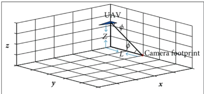
As schematically shown in Fig. 1, the irst two elements of Γ represent x and y positions of the footprint of the forward-looking camera. Also, the third element represents the altitude of the UAV. An important advantage of this scheme, compared to Kanchanavally et al. (2006), is that ϕ is not constant here and is considered one of the system state variables.
Assuming relative degree of ri for the i-th elements of Γ, ater ri times diferentiation, one inds:
and A3 = 0. Also:
where: Lf Γi is the Lie derivative, i.e. Lf Γi = ∂Γi/∂x and g i is
the i-th column of the matrix g. Also, A∈R3×1 and B∈R3×3, where the elements of Aare given below. For the system given by Eq. 1 and with output given by Eq. 2, one can obtain the vector of relative degree as [r1r2 r3] = [2 2 2].
One can verify that det(B) = –(x5)2cos x7/m·I·J sin3 x7 . his determinant can be zero if x5 = 0 or cosx7 = 0. In order to show that x5 ≠ 0, we deine the error as:
where: R is the reference signal and, for a stationary reference signal, one will have R = 0. Assuming E3(0) > −R3, one can rewrite the third row of Eq. 4 as:
herefore:
In the following paragraphs it will be shown that the absolute value of E3monotonically decreases and converges to zero. herefore, noting that R3 > 0, it will be easy to see that u’(t) is always positive. With Γ3(0) > 0, from Eq. 6, one can conclude that Γ3(t) > 0 and therefore x5 ≠ 0, i.e. the altitude cannot be zero. Also, for cosx7 = 0, one must have x7 = kn + π/2. It means that the objective position is exactly underneath the UAV actual position. his is an important drawback which can lead to the failure of this scheme. Yet, due to discretization, control errors and other real-world phenomena, this is not a concern in practical situations. In our simulations, no problem was encountered due to this drawback. Also, det(B) → ∞ if x7 → kπ. Yet, x7 → kπ means that L → ∞. In practice, it is not a legitimate concern because Γ3(0) > 0 and also the UAV cannot be ininitely far from its target (x7 ≠ kπ). herefore it is concluded that det(B) = –(x5)2cos x7/m·I·J sin3 x7 ≠ 0 for practical applications.
In order to study the error dynamics, we differentiate Eq. 4 to obtain:
Figure 1. The UAV and its camera footprint in scheme #1. z
x y
UAV
Z ϕ
L ϕ Camera footprint
∙
(2)(4)
(5)
Similar to Kanchanavally et al. (2006), if we define u = B–1(–A – Γ + υ) and , it is easy to see that:
where: K ∈ R3×3 and eigenvalues of K have negative real parts. In order to study the error dynamics given by Eq. 8, one may consider the following Lyapunov function:
he time derivative of the above positive deinite V is given by:
Therefore the error converges to zero. Regarding the internal dynamics with a vector of relative degree of [2 2 2], one needs to propose two more transformations to complete the difeomorphism. he internal dynamics is given by Eq. 11:
z
x y
UAV
Camera footprint L
Z ϕ
ϕ
Figure 2. The UAV and its camera footprint in scheme #2.
For the given output, one can verify that [r1r2r3] = [2 2 2]. Therefore, an equation identical to that given in Eq. 3 is obtained, in which:
One can verify that det(B) = –(x5)2cos x7/m·I·J sin3 x7. his determinant can be zero if x5 = 0 or cosx7 = 0. With the reasoning given in the previous subsection (see Eqs. 4 – 6), one can conclude that x5 ≠ 0, i.e. the altitude cannot be zero. For a UAV with constant forward velocity and a side-looking camera, the only possible motion where the error goes to zero is when the UAV loiters around the objective position, with a ixed loitering radius. herefore, with a non-zero loitering radius, it is easy to conclude that cosx7 ≠ 0. Also, det(B) → ∞ if x7 → kπ. Yet, x7 → kπ For a UAV with a forward-looking camera, the only possible
motion where the error goes to zero is when the UAV lies on a straight line over the objective position. herefore, as t → ∞, x4 → 0. With x4 → 0, it is easy to conclude that x3 will be bounded and therefore it is not going to cause undesirable efects. Simulation results verifying the feasibility of this approach will be given in “Simulations” section.
UAV with side-LooKing cAmerA, scheme #2
In this subsection, a UAV with variable-angle side-looking camera is considered. he equations of motion of this coniguration are identical to those given in Eq. 1 and therefore are not repeated here. For a side-looking camera, the output is given by:
∙
(7)
(8)
(12) (9)
(10)
(11)
means that L → ∞, which is not common in practical scenarios. herefore, it is concluded that det(B) = –(x5)2cos x7/m∙I∙J sin3 x7 ≠ 0 for practical applications, and thus the system given by Eq. 1 with output given by Eq. 12 is input-output linearizable.
For this scheme, the Lyapunov stability analysis is identical to that given by Eqs. 7 – 10. herefore, it can be concluded that the error dynamics asymptotically converges to zero. Regarding the internal dynamics with a vector of relative degree of [2 2 2], one needs to propose two more transformations to complete the difeomorphism. he internal dynamics is given by and in Eq. 13:
where the irst element of Γ is the square of the distance of the UAV from the origin of the coordinate system, i.e. the stationary objective position.
It can be readily seen that [r1r2r3] = [3 2 2]. herefore, in a compact form, one can write:
For a UAV loitering around a given objective position with constant (inite) forward velocity, x4 will be bounded and cannot go to ininity. Also, in a loitering motion, x3, i.e. the heading angle, can be shown by 2kπ + θ’ where θ’ is a inite value and therefore the internal dynamics will not cause undesirable efects in our approach. Simulation results regarding this scheme will be given in “Simulations” section.
An important drawback of this method is that one cannot explicitly control the inal loitering radius of the UAV. herefore, in the next scheme, we try to explicitly deine the loitering radius as one of the system outputs.
UAV with side-LooKing cAmerA, scheme #3
In this section, we modify the equations of motion given in Eq. 1 in a manner that a new useful scheme is obtained. In the control aine form, the new dynamic equations of motion are given by Eq. 14:
Here, the main difference is that L and L are explicitly considered to be state variables. One may deine the system output as:
where:
One can verify that det(B) = –2υc/m∙I (x1sinx3 – x2cosx3). An important disadvantage is that this determinant can be zero if x1sinx3 − x2cosx3 = 0, i.e. when the UAV is either lying radially inward or radially outward. Yet, if the heading of the UAV does not fall within this region, the UAV can converge to a loitering motion around the origin of the coordinate system. On the other hand, the advantage of this scheme is that, depending on the value of R1, i.e. the irst element of the reference signal, one can come up with scenarios in which the UAV converges to a loitering radius either smaller or greater than the initial one. Also, a second advantage is that one can explicitly control L, as R3. herefore, for R3 < 2 √R1, R3 = 22 √R1 and R3 > 2 √R1, one can deine scenarios in which the UAV loiters around the origin while the camera footprint sweeps a circle with the radius smaller than, equal to or greater than √R1. his is schematically shown in Figs. 3a to 3c.
Regarding the stability of the system, if we deine the error as:
∙
(13)
(15)
(16)
(14)
(17)
for a stationary reference signal, one will have R = R = 0 . Diferentiating Eq. 17, one has:
Now, if we deine u = B–1(–A – Γ + υ) and υ = KE, it is easy to see that:
where: K is a matrix with eigenvalues which have negative real parts.
In order to study the error dynamics given by Eq. 19, one may consider the following Lyapunov function:
Figure 3. Three different scenarios in scheme #3.
R 3 R
1 0. 5
loitering orbit
R
3
R
1 0.5
x y
z
UAV
Center of the loitering orbit
R 3
Camera footprint
Projection of the loitering orbit in UAV loitering orbit
UAV loitering orbit UAV loitering orbit
R 1 0.5
x x
y z
UAV
Center of the loitering orbit Center of the
Camera footprint x
y z
UAV
Camera footprint
x-y plane Projection of the loitering orbit in x-y plane
Projection of the loitering orbit in
x-y plane he time derivative of the above positive deinite V is given by:
Therefore the error dynamics is asymptotically stable. Regarding the internal dynamics with a vector of relative degree of [3 2 2], one needs to propose one more transformation to complete the difeomorphism. he internal dynamics is given by η8 in Eq. 22:
For a UAV loitering around a given objective position with constant (inite) forward velocity, x4 will be bounded and cannot go to ininity. herefore, the internal dynamics will not cause undesirable efects in our approach. Simulation results regarding this scheme will be given in “Simulations” section.
UAV with side-LooKing cAmerA And one VirtUAL ForwArd-LooKing cAmerA, scheme #4
In this subsection, we modify the previous scheme in the sense that the UAV can loiter around the origin with a desirable radius while avoiding the singularity problem of scheme #3. Convergence to a loitering radius (i) smaller or (ii) greater than the initial radius is studied separately.
Convergence to a Loitering Radius Smaller than the Initial One
In this scenario, it is initially assumed that the UAV is equipped with a virtual forward-looking camera. From geometry, one can find two tangent lines (and their corresponding tangency points) between the initial position of the UAV and the circle with the reference radius. In the irst phase, the UAV can choose one of the tangency points as its virtual objective position and ly over it, according to scheme #1, discussed earlier. Assuming that the UAV lies over the tangent line, its heading will be perpendicular to the radius of the objective circle as it reaches the virtual objective position. As the UAV reaches the tangency point, it switches to scheme #3. he advantage here is that, in the second phase, it is ensured that the heading of the UAV is far from inward-outward direction and therefore scheme #3 can bring the UAV to loiter around the objective position, with desirable radius. his is schematically shown in Fig. 4.
The details of feedback linearization, control laws and stability analysis of scheme #1 and scheme #3 were discussed in the previous subsections and are not repeated here. Simulation results of this scheme will be given in “Simulations” section.
∙
∙
(18)
(19)
(20)
(21)
(22)
(a)
(b)
x y
P h as e #1
Phase #2 Tangency point
V 0
x y
Phase #1
Phase #3
V
0
Phase #2
Tangency point
-2,000 -1,000
0 1,000
2,000
-4,000 -2,000 0 2,000 4,000
300 350 400 450 500
x [m] y [m]
z
[
m
]
0 100 200 300 400 500 600 0
50 100 150 180
T i me [s]
Ca
me
ra
a
n
gl
e [
de
g
]
Figure 4. Scheme #3, convergence to a loitering radius smaller than the initial one.
Figure 5. Scheme #3, convergence to a loitering radius greater than the initial one.
mass (kg)
moment of inertia — z-axis
(kg∙m2)
moment of inertia of the camera (kg∙m2)
Forward velocity
(m/s)
1 0.01 0.001 10
Table 1. Characteristics of the light ixed-wing UAV.
Convergence to a Loitering Radius Greater than the Initial One
Similar to the previous subsection, we assume that the UAV is equipped with a virtual forward-looking camera and a side-looking camera. he scenario proposed here consists of three phases, as shown in Fig. 5.
In the irst phase, based on scheme #1, the UAV lies to a virtual objective position which is on the extension of the line connecting the origin to the initial position of the UAV. Let’s denote the UAV distance from the origin by d and the desired loitering radius by R*. At the end of the irst phase, when d is relatively greater than R*, the UAV inds the tangent lines from its current position to the circle with the radius R*. With d relatively greater than R*, one can assume that, in the second phase, based on scheme #1, the UAV lies on the tangent line to reach the tangency point (second virtual objective position). Once at this point, the UAV has reached the reference radius and switches to scheme #3. In the third phase, based on scheme #3, the UAV loiters around the origin with R1= R*. he details of feedback linearization, control laws and stability analysis of scheme #1 and scheme #3 were discussed in the previous subsections and are not repeated here. Simulation results of this scheme will be given in “Simulations” section.
SIMULATIONS
In this section, some case studies are developed to verify the feasibility of the proposed schemes. A light ixed-wing UAV is considered, with its characteristics given in Table 1. In the simulations, where applicable, the initial condition of the UAV is assumed to be [−1,800 m 2,500 m 240 deg 1 deg/s 300 m 10 m/s 10 deg 1 deg/s]T . For the irst scheme, the reference signal
is assumed to be [100 m −20 m 500 m]T. For the described
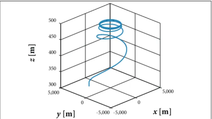
case study, simulations were carried out and the results are shown in Fig. 6.
As it can be readily seen from Fig. 6, after the initial transition, the UAV has aligned its motion such that it lies almost over the objective position on a straight line. Once on this line, the objective position is monitored by merely controlling the angle of the camera (see Fig. 7).
As it was expected, in this scheme, the camera angle will approach zero as the UAV lies toward the objective position. As the UAV lies away from the objective position, the camera angle will approach π, as t → ∞.
Figure 6. UAV trajectory obtained from scheme #1.
For the second scheme, the reference signal is assumed to be [−50 m −50 m 500 m]T. For the described case study,
simulations were carried out and the results are shown in Fig. 8. As it can be seen from Fig. 8, the UAV has successfully converged to a loitering motion around the objective position. Also, as expected, the camera angle converges to a fixed value in the loitering motion (see Fig. 9).
The initial conditions of the third scheme are assumed to be identical to those of the first scheme. Here, the reference signal is assumed to be [R0 500 m 30 deg]T, where R0 is the square distance of the UAV from the origin, at the initial time. Similar to the previous scenarios, simulations were carried out and the results are shown in Fig. 10.
Also, in this scheme, it is possible for the UAV to converge to a loitering circle with radius smaller/greater than the initial one. For the loitering radius of 1,500 and 4,500 m, simulations were carried out and the results are shown in Figs. 11 and 12, respectively. It can be seen from Figs. 11 and12 that the UAV has successfully converged to a loitering motion around the origin in both scenarios. Yet, it must be reminded that scheme #3 can fail if the UAV flies in the radial direction. Thus, it is recommended that one employs scheme #4 if a loitering motion is desirable.
It is important to note that scheme #4 includes scenarios where the loitering radius can be smaller/greater than the initial distance of the UAV from the origin.
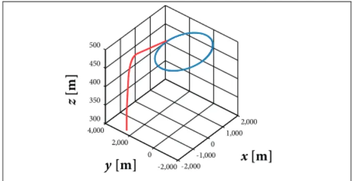
To verify the feasibility of scheme #4, a case study is developed in which the UAV is at the same initial condition as before. In the first example, let’s assume that the UAV is desired to loiter around the origin with a radius of 1,500 m, a value smaller than its initial distance to the origin. For this case study, simulation results are shown in Fig. 13.
Figure 8. UAV trajectory obtained from scheme #2.
Figure 9. Side-looking camera angle obtained from scheme #2.
-4,000 -2,000 0
2,000 4,000 -5,000 0 5,000 300 350 400 450 500 x[m]
y [m]
z
[
m
]
-5 ,0 0 0 0
5 ,0 0 0
-5 ,0 0 0 0 5 ,0 0 0 3 0 0 3 5 0 4 0 0 4 5 0 5 0 0
x[m]
y [m]
z [ m ] -5,000 0 5,000 -5,000 0 5,000 300 350 400 450 500 x[m]
y [m]
z [ m ] -5,000 0 5,000 -5,000 0 5,000300 350 400 450 500 x[m]
y [m]
z
[
m
]
0 500 1,000 1,500 2,000 2,500 3,000 3,500 4,000
9.9 9.95 10.0 10.05 10.1 10.15 10.2 10.25 10.3 Time [s] C ame ra a ngle [de g]
Figure 10. UAV trajectory obtained from scheme #3 — irst example.
Figure 11. UAV trajectory obtained from scheme #3 — second example.
-2,000 -1,000
0 1,000
2,000
-2,000 0 2,000 4,000 300 350 400 450 500
x [m] y [m]
z
[m
]
-5,000 0
5,000
-5,000 0 5,000 10,000 300 350 400 450 500
x [m]
y [m]
z
[m
]
In Fig. 13, the irst and the second phases of the path are shown in red and blue, respectively (see Fig. 4). As it can be seen from the igure, the UAV has successfully converged to the desired reference signal. In the second case study, assume that the UAV is desired to loiter around the origin with a radius of 4,000 m, a value greater than its initial distance to the origin. For this case study, simulation results are shown in Fig. 14, where the irst and the second phases of the path are shown in red and the last phase is shown in blue (see Fig. 5). As it can be seen from Fig. 14, the UAV has successfully converged to a loitering motion around the origin with the desired loitering radius.
CONCLUSION
In this paper, several feedback linearization schemes were studied to make a ixed-wing UAV, with constant forward velocity, (i) ly over or (ii) loiter around a stationary objective position. hroughout the paper, advantages and disadvantages of each scheme were discussed. A main drawback of the proposed schemes is that they do not take account of the maximum angular velocity constraint of ixed-wing UAVs. In scheme #1, the proposed method failed if the UAV was exactly above the objective position. Scheme #2 was disadvantageous in the sense that the loitering radius cannot be explicitly controlled. his was improved in scheme #3. Yet, the method in scheme #3 failed when the UAV had to ly radially inward or radially outward. However, if the heading of the UAV did not fall within this region, the UAV converged to a loitering motion around the origin. In scheme #4, the UAV had to be far enough from the objective circle. In this manner, one could assume that the UAV reaches the tangency point with its heading far from inward-outward direction, and therefore scheme #3 could bring the UAV to loiter around the objective position, with desirable radius. It is important to note that, in scheme #3 and scheme #4, the switching from a control strategy to another was given as an equality-type condition. herefore, for real-world implementation, thresholds must be deined, and the equalities must be replaced by appropriate inequalities.
ACKNOWLEDGEMENTS
he authors gratefully acknowledge the inancial support of Conselho Nacional de Desenvolvimento Cientíico e Tecnológico (CNPq), Financiadora de Estudos e Projetos (FINEP), Fundação de Amparo à Pesquisa do Estado de Minas Gerais (FAPEMIG) and Coordenação de Aperfeiçoamento de Pessoal de Nível Superior (CAPES), Brazil.
Figure 13. UAV trajectory obtained from scheme #4 — irst case study.
Figure 14. UAV trajectory obtained from scheme #4 — second case study.
REFERENCES
Almurib HAF, Nathan PT, Kumar TN (2011) Control and path planning of quadrotor aerial vehicles for search and rescue. Proceedings of the IEEE SICE Annual Conference; Tokyo, Japan.
Beard RW, McLain TW, Nelson DB, Kingston D, Johanson D (2006) Decentralized cooperative aerial surveillance using ixed-wing miniature UAVs. Proc IEEE 94(7):1306-1324. doi: 10.1109/ JPROC.2006.876930
Bonyan Khamseh H, Pimenta LCA, Tôrres LAB (2014) Decentralized coordination of constrained ixed-wing unmanned aerial vehicles: circular orbits. Proceedings of the IFAC World Congress; Cape Town, South Africa.
Costa FG, Ueyama J, Braun T, Pessin G, Osório FS, Vargas PA (2012) The use of unmanned aerial vehicles and wireless sensor network in agricultural applications. Proceedings of the IEEE International Geoscience and Remote Sensing Symposium; Munich, Germany.
Fan W, Zhiyong G (2009) An approach to formation maneuvers of multiple nonholonomic agents using passivity techniques. Proceedings of the Chinese Control and Decision Conference; Guilin, China.
Frew E, Lawrence D, Morris S (2008) Coordinated standoff tracking of moving targets using Lyapunov guidance vector ields. J Guid Contr Dynam 31(2):290-306. doi: 10.2514/1.30507
Gonçalves MM, Pimenta LCA, Pereira GAS (2011) Coverage of curves in 3D with swarms of nonholonomic aerial robots. Proceedings of the IFAC World Congress; Milano, Italy.
Gonçalves VM, Pimenta LCA, Maia CA, Dutra BCO, Pereira GAS (2010) Vector ields for robot navigation along time-varying curves in n-dimensions. IEEE Trans Robot26(4):647-659. doi: 10.1109/ TRO.2010.2053077
Hafez AT, Marasco AJ, Givigi AN, Beaulieu A, Rabbath CA (2013)
Encirclement of multiple targets using model predictive control. Proceedings of the American Control Conference; Washington, USA.
Hsieh MA, Kumar V, Chaimowicz L (2008) Decentralized controllers for shape generation with robotic systems. Robotica 26(5):691-701. doi: 10.1017/S0263574708004323
Hsieh MA, Loizou S, Kumar RV (2007) Stabilization of multiple robots on stable orbits via local sensing. Proceedings of the IEEE International Conference on Robotics and Automation; Rome, Italy.
Kanchanavally S, Ordonez R, Schumacher CJ (2006) Path planning in three dimensional environment using feedback linearization. Proceedings of the American Control Conference; Minneapolis, USA.
Li H, Wang B, Liu L, Tian G, Zheng T, Zhang J (2013) The design and application of SmartCopter: an unmanned helicopter based robot for transmission line inspection. Proceedings of the Chinese Automation Congress; Changsha, China.