ABSTRACT: The work is a study of conservation on linearization techniques of time-marching schemes for the unstructured inite volume Reynolds-averaged Navier-Stokes formulation. The solver used in this work calculates the numerical lux applying an upwind discretization based on the lux vector splitting scheme. This numerical treatment results in a very large sparse linear system. The direct solution of this full implicit linear system is very expensive and, in most cases, impractical. There are several numerical approaches which are commonly used by the scientiic community to treat sparse linear systems, and the point-implicit integration was selected in the present case. However, numerical approaches to solve implicit linear systems can be non-conservative in time, even for formulations which are conservative by construction, as the inite volume techniques. Moreover, there are physical problems which strongly demand conservative schemes in order to achieve the correct numerical solution. The work presents results of numerical simulations to evaluate the conservation of implicit and explicit time-marching methods and discusses numerical requirements that can help avoiding such non-conservation issues.
KEYWORDS: Computational luid dynamics, Time marching methods, Flux vector splitting scheme, Conservative discretization.
Study of Conservation on Implicit
Techniques for Unstructured Finite
Volume Navier-Stokes Solvers
Carlos Junqueira-Junior1, Leonardo Costa Scalabrin2, Edson Basso3, João Luiz F. Azevedo3
INTRODUCTION
his work discusses issues associated with the coupling of implicit integration methods, for unstructured inite volume formulations, with the spatial discretization based on flux vector splitting schemes. he material discussed in the work is an extension of the work of Barth (1987). he original paper discussed the approximate local time linearizations of nonlinear terms for the inite diference formulation using Total Variation Diminishing (TVD) (Harten, 1983) and upwind algorithms. Here, the time conservation of the point-implicit integration for unstructured meshes is analyzed and discussed. Finite volume formulations have the tremendously important property of being conservative by construction. However, some time integration approaches may present numerical issues that can destroy this property, at least for unsteady applications or during the process of converging to a steady state. his shortcoming was observed when performing simulations of the low inside closed systems in which there is no addition or extraction of luid mass to/from the system. For such systems, the use of the point-implicit schemes discussed in this present paper has led to heat generation and non-conservation of mass in the interior of the computational domain. Results of simulations using explicit and implicit integration methods are presented in the present paper in order to better understand the non conservation issue of the time-marching methods. An analysis of the problem is also performed by a detailed study of the backward Euler method linearization.
1.Instituto Tecnológico de Aeronáutica – São José dos Campos/SP – Brazil 2.EMBRAER S.A.– São José dos Campos/SP – Brazil 3.Instituto de Aeronáutica e Espaço – São José dos Campos/SP – Brazil
Author for correspondence: João Luiz F. Azevedo | Instituto de Aeronáutica e Espaço | Praça Eduardo Gomes, 50 – Vila das Acácias | CEP: 12228-901 São José dos Campos/SP – Brazil | Email: [email protected]
THEORETICAL FORMULATION
h e formulation used in the present work is based on the Reynolds-averaged Navier-Stokes set of equations, also known by the Computational Fluid Dynamics (CFD) community as the Reynolds Averaged Navier-Stokes (RANS) equations. h e RANS equations are obtained by time i ltering the Navier-Stokes set of equations. h e compressible RANS equations are written in the algebraic vector form as
. (1)
h e conserved variables vector, Q, the inviscid l ux vector, Fe, and the viscous l ux vector, Fv, are given by
, (2)
, (3)
, (4)
in which ρ stands for density, for the velocity vector in Cartesian coordinates, p for static pressure, τ for viscous stress tensor, qH for heat l ux vector, e for the total energy per unit volume and βi is given by
. (5)
he îx, îy and îz terms are the Cartesian-coordinate orthonormal vector basis. It is very important to emphasize that i eld forces, such as gravity, are neglected here.
Other equations are necessary in order to close the system of equations given by Eq. (4). h ese additional equations are called constitutive relations. h e i rst constitutive equation
presented to close the Navier-Stokes set of equations is known as the equation of state. h is equation considers the perfect gas law, and it is written as
, (6)
in which the mean total energy per unit volume, e, is given by
, (7)
and ei stands for internal energy, dei ned as
, (8)
in which T stands for the mean static temperature and Cv is the specii c heat at constant volume. h e heat l ux from Eq. (5) is obtained from the Fourier law for heat conduction, and it is given by
, (9)
in which γ is the ratio of specii c heats and Pr is the Prandtl number. Typically, for air, it is assumed that γ = 1.4 and
Pr = 0.72. Cp is the gas specii c heat at constant pressure and μ
is the dynamic molecular viscosity coeffi cient, calculated as a function of the temperature by the Sutherland law equation (Anderson, 1991), written as
, (10)
where S = 110K , and µ
∞ is the dynamic molecular viscosity
coeffi cient of the l uid at temperature T∞.
h e components of the viscous stress tensor, for a Newtonian l uid, are given by
, (11)
in which δij stands for the Kronecker delta.
NUMERICAL FORMULATION
RANS equations discretized in the context of a cell-centered finite-volume. The solver used in the present work is Le Michigan Aerothermodynamics Navier-Stokes Solver (LeMANS). h e original framework was developed by Scalabrin (2007) at the University of Michigan to simulate hypersonic l ows over reentry capsules. It is a three dimensional (3-D) numerical solver that uses the i nite volume formulation for unstructured meshes to solve the RANS equations coupled with non-equilibrium chemical reaction equations and the Spalart-Allmaras (SA) turbulence model (Spalart and Allmaras, 1992; 1994). h e numerical l ux is calculated using an upwind scheme based on the Steger-Warming l ux vector splitting (Steger and Warming, 1981). h e time integration is performed by point implicit and Runge-Kutta methods. h is section describes the numerical formulations and discretizations applied in the present work.
FINITE VOLUME FORMULATION
The finite volume formulation is a numerical method applied to represent and evaluate partial dif erential equations. It is applied by the CFD community to i nd the solution of the RANS, equations. h e method is obtained integrating the l ow equations for each control volume within a given mesh. h e RANS equations, written in the context of a cell-centered i nite-volume formulation, are given by
. (12)
Considering a cell-centered formulation, Viis a given cell of the given grid. At er the integration it is possible to apply the Gauss theorem over the equation above, resulting in:
, (13)
in which Siis the outward-oriented area vector and it is dei ned as
. (14)
Considering the mean value of the conserved variables within the i-th control volume, one can write the i rst term of Eq. (13) as
. (15)
h e second term of Eq. (13) can be written as the sum of all faces of a cell
, (16)
in which the k subscript is the index of the cell face, and nf
indicates the number of faces of the i-th volume. Finally, the RANS equations discretized with a i nite volume approximation are given by
. (17)
For this formulation, the l uxes are computed at the faces of the control volume, and the conserved variables are computed in the cell.
INVISCID FLUX CALCULATION
h e inviscid l uxes are calculated using a method based on a classical l ux vector splitting formulation, the Steger-Warming Scheme (SW) (Steger and Warming, 1981). h is method is an upwind scheme which uses the homogeneous property of the inviscid l ux vectors to write
, (18)
where Fen is the normal flux at the k-th face, and A is the Jacobian matrix of the inviscid l ux which can be diagonalized by the matrices of its eigen vectors from the let and from the right, L and R
A = R Λ L , (19)
and Λ is the diagonal matrix of the eigenvalues of the Jacobian matrix. h e A matrix can be split into positive and negative parts as
A+ = R Λ+L and A− = R Λ−L . (20)
h e splitting separates the l ux into two parts, the downstream and the upstream l ux, in relation to the face orientation as:
, (21)
where the cl and cr subscripts are the cells on the let and right sides of the face. h e split eigen values of the Jacobian matrix are given by
In order to avoid sudden sign transition, and then discontinous derivative, the split eigen values receive a small number, ε , turning Eq. (22) into
. (23)
h e sot en sign transition turns the derivative continous at the transition point.
Numerical studies performed in the present work indicated that this flux vector splitting is too dissipative and it can deteriorate the boundary layer profiles (Junqueira- Junior, 2012; Junqueira-Junior et al., 2013; MacCormack and Candler, 1989). Therefore, a pressure switch is implemented to smoothly shift the Steger-Warming scheme into a centered one. Then, the artificial dissipation is controlled and the numerical stability is maintained, as presented in the following formulation:
. (24)
in which
(25)
h e switch, w, is given by
, (26)
where ∇p is a scalar number, a numerical approximation of the pressure gradient. For small ∇p, = (1 − ) = 0.5, the code runs with a centered scheme, and for larger values of ∇p, = 0 and (1 − ) = 1, the code runs with the original Steger-Warming scheme. For Eq. (26) one suggests α = 6, but some problems may require larger values (Scalabrin, 2007).
h e applied formulation was originally created with interest on studying l ows over reentry capsules. For such particular cases, with very strong shock waves, it is very common to i nd solutions with numerical and non-physical structures such as carbuncles (Ramalho et al., 2011). To avoid such numerical problems, artii cial dissipation has to be added to the method. h e dissipation was included into the split eigenvalues, Eq. (23), using an ε factor, which is given by:
(27)
where dkis the distance of the k-th face, to the nearest wall boundary. d0 is set by the user and must be smaller than the boundary layer thickness and larger than the shock stand-off distance. is the normal vector of the nearest wall, and is the normal vector to the k-th face. Equation (27) applies the term to decrease the value at the faces parallel to the wall inside the boundary layer (Scalabrin, 2007). This artificial dissipation model has shown an important role in the prediction of boundary layer profiles (Junqueira-Junior, 2012; Junqueira-Junior
et al., 2013).
VISCOUS FLUX CALCULATION
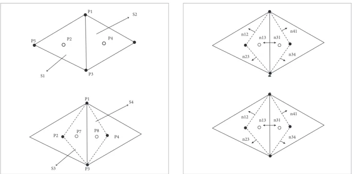
h e viscous terms are based on derivative of properties on the faces. To build the derivative terms, two volumes are created over the face where the derivative is being calculated. At the center of each new volume, the derivative is calculated using the Green-Gauss theorem. h is computation is used to i nd the derivative at the desired face.
A two dimensional (2-D) example is used in this section to better explain the derivative calculation. Consider the two cells, S1 and S2, in Fig. 1. Two new cells, S3 and S4, are created using node points, P1 and P3, and cell centered points, P2 and P4, to calculate the derivative on 1-3 face. h e properties at the faces are calculated using simple averages. For example, in Figs. 1 and 2, the properties are given by
(28)
. (29)
Considering ∇Q as a constant over the cell, the equation above yields
in which ∇Q is the constant cell-centered gradient. Using the derivatives in the S3 and S4 cells, the derivative at faces 1-3 is computed using
. (31)
The derivative computation for other types of element, 2-D or 3-D, is straightforward.
TIME INTEGRATION
h e explicit second-order Runge-Kutta (Lomax et al., 2001) and the point implicit scheme are the two time-marching methods applied in the present work.
h e second-order Runge-Kutta integration method used in this work is given by
(32)
In order to simplify the forthcoming equations, the right hand side of Eq. (32) is written as
(33)
in which Rcl is the residue of the i-th cell.
h e implicit integration applied in the present work is based on the backward Euler method, which is given by
. (34)
One can linearize the residue at time n + 1 as a function of properties at time n.
, (35)
P1
P2
P3 P4 P5
S1
S2
P1
P7 P8
P3
P4 P2
S3
S4
Figure 1. 2-D example of new volume creation. Figure 2. 2-D example of derivative calculation.
n12 n41
n34 n23
n13 n31
n12 n41
n34 n23
From the spatial discretization, the inviscid terms can be written as
(36)
It is a common practice to assume
, (37)
and then write
(38)
which is not true and different from the real definition of the Jacobian matrix written in Eq. (20). Using the approximate form, Eq. (38) to calculate the inviscid terms may decrease the numerical stability of the method. Hence, in this work, the true Jacobian matrices of the split fluxes, given by Eq. (20), are implemented in order to calculate the implicit operator. The approximate Jacobian matrices, which are calculated using Eqs. (37) and (38), are implemented at the right hand side of the linear system. Issues involving the true Jacobians matrices have a major importance in the context of numerical stability for computational methods (Anderson et al., 1986; Hirsch, 1990; Steger and Warming, 1981).
h e viscous terms can be written in the same form as
(39)
In this work, the viscous Jacobian matrices are represented by
B. Hence, the Jacobian matrix splitting is written as
. (40)
One can write the system as
(41)
It is, then, possible to write
, (42)
with
, (43)
. (44)
and
. (45)
As the code is an unstructured solver, this system of equations results in a sparse block matrix, where each block is a square matrix of size equal to the number of equations to be solved in each control volume. h e solution of such system is typically very expensive and, depending on the size of the mesh, it is not even practical. A less expensive implicit method is applied in the present work, the implicit point integration (Gnof o, 2003; Venkatakrishnan, 1995; Wright, 1997).
h e main idea of the implicit point integration is to move all the of -diagonal terms to the right hand side and to solve the resulting system iteratively, i.e.,
. (46)
It is assumed that ∆Qn+1.0 = 0 and four iterations are taken in the
where each ☐ is a 5 × 5 block matrix. h e time step is computed by
, (47)
in which CFL is a parameter set to ensure the stability of the time integration method, l is the size of the cell and
is the largest wave speed in the cell.
BOUNDARY CONDITIONS
h e boundary conditions are implemented using ghost cells. h e solver creates the ghost cells to hold properties that satisfy the correct l ux calculation at the boundaries. h e implementation assigns properties that satisfy the Euler boundary conditions to calculate the inviscid l uxes, and properties that satisfy the Navier-Stokes boundary conditions to calculate the viscous l uxes. h erefore, the ghost volumes store two dif erent types of l uxes for the correct computation of the RANS equations.
WALL INVISCID BOUNDARY CONDITIONS
h e ghost cells hold the properties in the same manner to calculate the inviscid l uxes at the wall and at the symmetry boundaries. Mass and energy l uxes should yield zero, and the momentum flux is equal to the pressure flux. This is accomplished by setting the normal velocity component to the boundary face zero. In the present work, the interior domain
is dei ned as the properties at the let side of the boundary face and the ghost cells are dei ned as the properties at the right side of the boundary.
In order to simplify the implementation, the properties at the let side of the boundary face are rotated to the face coordinates using
. (48)
h e vector of conservative properties, Q, is written as
(49)
In Eq. (48), is the rotation matrix given by,
(50)
and the vectors define the face-based reference frame. h e properties at the ghost cells are set to
(51)
One can write in the matrix form as
, (52)
in which is the inviscid wall matrix given by
. (53)
h erefore, the boundary condition can be written as
in which the R−1 matrix is given by
. (55)
It returns the properties to the Cartesian coordinate frame.
VISCOUS WALL BOUNDARY CONDITION WITH SPECIFIED TEMPERATURE
Viscous wall with specii ed temperature does not have necessarily zero heat conduction at the boundary face. For this boundary condition the user provides the wall temperature, Twall , and the wall pressure is extrapolated from the interior in order to satisfy the zero normal wall pressure gradient condition Schlichting (1978). Hence,
(56)
One can computate the conservative properties at the wall boundary using the Cartesian components of the wall velocity,
and , which are set by the user.
(57)
h en, the ghost cell conservative properties are calculated using an average between the let and right cells
(58)
IMPLICIT BOUNDARY CONDITIONS
Implicit boundary conditions are necessary in order to obtain a truly implicit time-marching method. h e use of explicit boundary
conditions can limitate substantially the stability of the numerical method in the marching procedure for the solution convergence.
BASIC IMPLICIT FORMULATION
A simplified form of the implicit equation, Eq. (42), is written in this section in order to detail the implementation of implicit boundary conditions for l ux vector splitting schemes,
(59)
where the repeated k index, in the second term in let hand side of the equation, indicates summation over all the k faces of the control volume. h e equation above is written only to present the relation between an internal cell, cl, and a boundary cell, cr, k. In the original formulation, Eq. (42), the cl-th cell has contributions from other faces, which may or may not be boundaries.
As discussed in the present work, the ghost cells hold dif erent values for inviscid and viscous calculations. Hence, using the splitting dei nition, presented in section Inviscid Fluxes Calculation, Eq. (59) can be written as
(60)
h e contributions of the boundary face can be expressed in terms of the internal cell corrections as
(61)
Hence, Eq. (60), can be rewritten as
(62)
h e viscous Jacobians are calculated using primitive variables, then the corrections are set for the primitive variables and applied directly at the calculation of the viscous Jacobians. h e matrix B+
k+
already includes the contribution from the boundary. h e A+
k+ ,
A−
k- , B +
k+ and B −
INVISCID WALL MATRICES FOR IMPLICIT BOUNDARY CONDITIONS
h e matrix for an inviscid wall or for a symmetry boundary is the same matrix presented in Eq. (54),
k, inv, wall
=
-1
W
.
(63)The matrices are applied to ∆Q for the implicit boundary condition according to Eq. (61).
VISCOUS WALL WITH SPECIFIED TEMPERATURE MATRIX FOR IMPLICIT BOUNDARY CONDITIONS
h e viscous Jacobians are created using primitive variables. Hence, the implementation of implicit viscous matrices is performed using primitive variables. h ey are applied directly at the calculation of the Jacobians matrices.
h e code was originally created for l ow simulation with chemical reactions, hence the mass fraction, Y , is present in the primitive variable vector, which is given by
. (64)
In the present work, it is always considered that there is only one species in the l ow, then, Y = 1.
h e implicit matrix for wall boundary with specii ed temperature is derived from the average between the let and right cells,
, (65)
in which z is given property. h e velocity components and temperature at the wall are considered constants in time, hence,
. (66)
h e mass fraction, Y, at the wall, is given by the let cell value,
Ywall = Ycl . h erefore, the implicit matrix for wall boundary with specii ed temperature is given by
.
(67)
CONSERVATION ANALYSIS OF
IMPLICIT METHODS
GENERAL CONSERVATION ANALYSIS
At er this brief review, the backward Euler time marching method, Eq. (42), is re-written using a simplii ed notation
. (68)
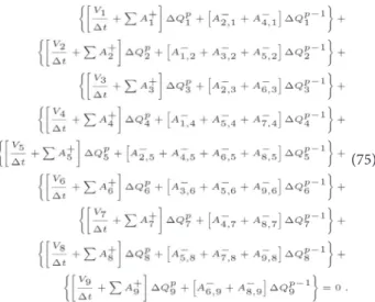
The integration is applied on a generic grid, which is a representative 2-D i nite volume mesh using nine quad-cells, as illustrated in Fig. 3, in order to present the conservative issues of such linearization. h e [M] matrix, for the mesh used here, is represented by
(69)
h e formulation can be considered conservative when the sum of Vi ∆Qin terms, for all cells, yields zero, i.e.,
, (70)
or yet
. (71)
(72)
It is possible to simplify this equation in order to write
, (73)
where the [Ci ] matrix is the sum of the inviscid and viscous Jacobian matrices in each column of the [M] matrix. Comparing Eqs. (71) and (73), one can easily state that, in order to preserve the conservative property of the i nite volume formulation, the [Ci ] matrices should be zero and ∆tshould be the same for all the cells in the domain, i.e.,
. (74)
POINT IMPLICIT CONSERVATION ANALYSIS
If one solves the linear system for the same mesh presented in Fig. 3 using the point-implicit integration, after a converged solution is obtained, i.e., Rin = 0, one
could finally write
(75)
One can state that, as long the sub-iterations of the point implicit method have not achieved the convergence for ∆Qip
and/or ∆t is not the same for all the cells in the domain, it is not possible to i nd a general relation for any ∆ Qip and ∆ Q
i p−1 such
that ∑ [Vi ∆Qin ] = 0. h erefore, the conservation property for
the point-implicit integration can be achieved only if the [Ci ] matrices are zero, the solution of ∆Qip for the sub-iterations in
p is converged, and ∆t is constant over the entire mesh. However, achieving convergence of the point-implicit sub-iterations can be as expensive as performing the fully implicit integration. Hence, all practical numerical solvers perform a limited number of sub-iterations. h e authors, usually, perform up to 10 sub-iterations in p for the point-implicit integration and, then, move on to the next time step. Typically, this is not enough to achieve convergence for ∆Qip, as discussed the
forthcoming section of the paper.
RESULTS AND DISCUSSION
Results for the so-called “rigid body simulation” problem are presented in this section in order to expose the ef ects of the time-marching scheme on the mass conservation. h e rigid body problem consists of the simulation of the l ow contained between two concentric cylinders, in which both walls rotate at the same angular velocity. h erefore, at er convergence, the l uid in the domain is rotating at the same angular velocity as if it were a rigid body. Here, the problem is addressed as a 2-D l ow. h e present work performed simulations using the point-implicit and the Runge-Kutta time marching methods.
An analysis of the use of a constant CFL number on all mesh cells is also presented here, in comparison to the use of a constant
Δt throughout the mesh.
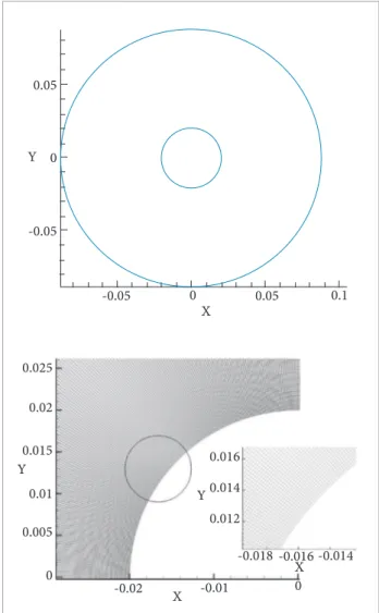
h e two dimensional geometry and the detailed 360,000 cell mesh, used in the simulations, are presented in Fig. 4. h e external and internal cylinders are rotating walls with i xed angular velocity, ω, and i xed temperature, T0. Air with zero velocity and T0 temperature are considered as initial conditions. All simulations are conducted with the same initial and boundary conditions. Each simulation is performed using a dif erent time marching method, as presented in Table 1.
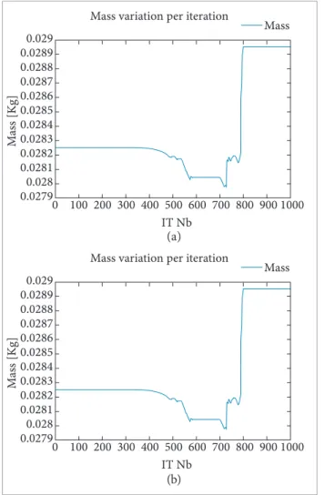
Figures 5 and 6 present the total amount of mass (per unit of length in the cylinder axial direction) inside the computational domain, as a function of the iteration number, for the rigid body simulations. It is clear from the i gures that the point implicit time marching method can signii cantly deteriorate the important conservative property of the i nite volume formulation. Moreover, both simulations with the point-implicit time-marching scheme presented exactly the same non-conservative behavior. Moreover, for the point-implicit time integration test cases, i.e., test cases 1 and 2, or cases shown in Fig. 5 (a) and (b), there is almost no inl uence of the selection of constant CFL or of constant ∆t in the time march. In other words, one could state that, for these test cases, the non-conservation ef ects of using a constant CFLnumber are far less signii cant than the ef ects of using the point implicit integration. Furthermore, it is correct to state that both simulations diverged at er some time (not shown in Fig. 5 (a) and (b).
In contrast to that behavior, simulations performed using the explicit Runge-Kutta scheme and a constant time step throughout the domain perfectly conserve the mass in the computational domain, as one would expect from a i nite volume code. h e results for this test case (case 4) are shown in Fig. 6 (b). On the other hand, results in Fig.6 (a) indicate that, even with an explicit scheme, there is no mass conservation if a variable time step, or constant CFL number, is used in the time integration. h is is a serious problem since most convergence acceleration procedures typically employed in aerospace CFD codes are based on the use of implicit integration or on variable time stepping, or both. h e present results are clearly demonstrating that, for such cases, there is no mass conservation during the transient process of converging to a steady state solution.
Moreover, all results presented in Figs. 5 and 6 reinforce the previous analysis performed in this work. To assure the conservative property of a time marching method, the [Ci ]
matrix should be zero. h is is automatically enforced by the explicit integration schemes by construction. h erefore, for the point implicit integration, the convergence of the sub-iterations has to be achieved in order to obtain a conservative scheme. Furthermore, all the mesh cells have to advance in time using
0.05
0.05 0.1
0 X Y
-0.05
-0.05 0
0.005
0.015 0.016
-0.016 0.014
-0.014 -0.018
0.012 0.025
0.01 0.02
0
X
X
-0.02 -0.01 0
Y
Y
Figure 4. Rigid body geometry and mesh detail.
Table 1. Dei nition of the test case coni gurations for the numerical simulations.
Case Time marching scheme Constant ∆t or CFL
1 Point implicit Constant CFL
2 Point implicit Constant ∆t
3 Runge-Kutta Constant CFL
the same ∆t value in order to maintain the conservative property of the inite volume method. his is true even for the explicit time marching methods.
CONCLUSIONS
A discussion on the issues associated with the coupling of implicit integration methods, for unstructured inite volume formulations, with the spatial discretization based on lux vector splitting schemes, is presented in this work. he linearization of inviscid and viscous Jacobians may result in a non-conservative method during the transient phase of the low simulation, even for the finite volume formulation, which is supposed to be
conservative by construction. he present analysis of the numerical formulation and of the computational results obtained has indicated that the time integration can be considered conservative only if the sum of the Jacobian matrices in each column of the linear system matrix is zero and all mesh cells have the same ∆t value. Moreover, very popular approximate methods used in many CFD codes, to solve sparse linear systems, such as the point implicit integration, need to achieve convergence of the sub-iterations in order to be conservative during the transient portion of the simulation. his is a very expensive proposition and it can make such approximate solvers as expensive as those which perform the direct solution of the full implicit linear system.
he important conclusion is that care must be exercised in the linearization of time-marching methods for simulations which demand the conservative property. It is important to
0.029 0.0289 0.0288 0.0287 0.0286 0.0285 M as s [K g] Mass Mass variation per iteration
IT Nb
0 100 200 300 400 500 600 700 800 900 1000 0.0284 0.0283 0.0282 0.0281 0.028 0.0279 1.2 1 0.8 0.6 0.4 0.2 0 M as s [K g ] Mass
Mass variation per iteration
2nd ord. Runge-Jutta constant DCF
IT Nb
0 500 1000 1500 2000 2500 3000 3500 4000
0.029 0.0289 0.0288 0.0287 0.0286 0.0285 M as s [ K g] Mass
Mass variation per iteration
IT Nb
0 100 200 300 400 500 600 700 800 900 1000 0.0284 0.0283 0.0282 0.0281 0.028 0.0279 0.02826 0.028258 0.028256 0.028254 0.028252 0.02825 0.028248 0.028246 0.028244 0.028242 0.02824 M as s [ K g] Mass
Mass variation per iteration
2nd ord. Runge-Jutta constant CFL
IT Nb
0 1000 2000 3000 4000 5000 6000
Figure 5. Effects of implicit time marching scheme on total mass conservation; (a) Constant CFL calculation for point-implicit scheme; (b) Constant ∆t calculation for point-implicit scheme.
Figure 6. Effects of explicit time marching scheme on total mass conservation; (a) Constant CFLcalculation for explicit RK scheme; (b) Constant ∆t calculation for explicit RK scheme.
(a)
(b)
(a)
be aware of the efects of such issue on the physical problem of interest. Physical problems with incoming and outcoming low boundary conditions, very common in simulations for aerospace applications, do not necessarily need a conservative scheme during the transient portion of a steady state calculation. he amount of variation in the low properties, during one time step, is negligible compared to the lux of the same properties that is crossing the open boundaries of the domain. Moverover, for many steady-state external aerodynamic applications, the initial conditions are strictly numerical, in the sense that they cannot be physically realized as implemented in the solver. In other words, they are typically associated to impulsively started lows. For such cases, the aspect of the lack of mass conservation in the entire computational domain, as the solution evolves from a non-physical initial condition to a physically relevant converged steady state condition, is not an issue. On the other hand, the conservative property is absolutely essential for closed systems, in which the total mass, and other properties, must always be
conserved in order to achieve a physically relevant solution. In these critical cases, approximate numerical methods should not be used in order to solve the full implicit linear systems.
ACKNOWLEDGEMENTS
he authors would like to acknowledge Conselho Nacional de Desenvolvimento Cientíico e Tecnológico, CNPq, which partially supported the project under the Research Grant No. 309985/2013-7. Partial support for the present research was also provided by Fundação de Amparo à Pesquisa do Estado de São Paulo, FAPESP, under Research Grants No. 2013/07375 and No. 2013/21535-0. Further partial support was provided by Fundação Coordenação de Aperfeiçoamento de Pessoal de Nível Superior, CAPES, through a Ph.D. scholarship to the irst author, which is also gratefully acknowledged.
REFERENCES
Anderson, J.D.J., 1991, “Fundamentals of Aerodynamics”, McGraw- Hill International Editions, New York, NY, USA.
Anderson, W.K., Thomas, J.L. and Van Leer, B., 1986, “A Comparison of Finite Volume Flux Vector Splittings for the Euler Equations”, AIAA Journal, Vol. 24, No. 6, pp. 1453–1460.
Barth, T.J., 1987, “Analysis of Implicit Local Linearization Techniques for Upwind and TVD Algorithms”, Proceedings of the 25th AIAA Aerospace Sciences Meeting, AIAA Paper No. 87-0595, Reno, NV, USA.
Gnoffo, P.A., 2003, “Computational Aerothermodynamics in Aeroassist Applications”, Journal of Spacecraft and Rockets, Vol. 40, No. 3, pp. 305–312. doi: 10.2514/2.3957.
Harten, A., 1983, “High Resolution Schemes for Hyperbolic Conservation Laws”, Journal of Computational Physics, Vol. 49, No. 3, pp. 357–393. doi: 10.1016/0021-9991(83)90136-5.
Hirsch, C., 1990, “Numerical Computation of Internal and External Flows”, Vol. 2, Computational Methods for Inviscid and Viscous Flows, John Wiley and Sons, New York, USA.
Junqueira-Junior, C.A., 2012, “A Study on the Extension of an Upwind Parallel Solver for Turbulent Flow Applications” Masters Thesis, Instituto Tecnológico de Aeronáutica, São José dos Campos, SP, Brasil.
Junqueira-Junior, C.A., Azevedo, J.L.F., Scalabrin, L.C. and Basso, E., 2013, “A Study of Physical and Numerical Effects of Dissipation on Turbulent Flows Simulations”, Journal of Aerospace Technology and Management, Vol. 5, No. 2, pp. 145–168. doi: 10.5028/jatm.v5i2.179.
Lomax, H., Pulliam, T.H. and Zingg, D.W., 2001, “Fundamentals of Computation Fluid Dynamics”, Springer, NY, USA.
MacCormack, R.W. and Candler, G.V., 1989, “The Solution of the Navier-Stokes Equations Using Gauss-Seidel Line Relaxation”, Computer and Fluids, Vol. 17, No. 1, pp. 135–150. doi: 10.1016/0045-7930(89)90012-1.
Ramalho, M.V.C., Azevedo, J.L.F. and Azevedo, J.H., 2011, “Further Investigation into the Origin of the Carbuncle Phenomenon in Aerodynamic Simulations”, 49th AIAA Aerospace Sciences Meeting Including the New Horizons Forum and Aerospace Exposition, AIAA Paper No. 2011-1184, Orlando, FL, USA.
Scalabrin, L.C., 2007, “Numerical Simulation of Weakly Ionized Hypersonic Flow Over Reentry Capsules”, PhD Thesis, Department of Aerospace Engineering, The University of Michigan, Michigan, USA.
Schlichting, H., 1978, “Boundary-Layer Theory”, 7th Edition, McGraw Hill, New York, USA.
Spalart, P.R. and Allmaras, S.R., 1992, “A One-Equation Turbulence Model for Aerodynamic Flows”, Proceedings of the 30th AIAA Aerospace Sciences Meeting and Exhibit, AIAA Paper No. 92–0439, Reno, NV, USA.
Spalart, P.R. and Allmaras, S.R., 1994, “A One-Equation Turbulence Model for Aerodynamic Flows”, La Recherche Aerospatiale, Vol. 1, pp. 5–21.
Steger, J.L. and Warming, R.F., 1981, “Flux Vector Splitting of the Inviscid Gasdynamic Equations with Application to the Finite-Difference Method”, Journal of Computational Physics, Vol. 40, No. 2, pp. 263– 293. doi: 10.1016/0021-9991(81)90210-2.
Venkatakrishnan, V., 1995, “Implicit Schemes and Parallel Computing in Unstructured Grid CFD”, Technical Report, ICASE Report No. 95-28, ICASE.
ABBREVIATIONS
2-D: Two dimensional
3-D: Three dimensional
CFD: Computational Fluid Dynamics
CFL: Courant-Friedrichs-Lewy number
LeMANS: Le Michigan Aerothermodynamics Navier- Stokes Solver
RANS: Reynolds Averaged Navier-Stokes
SA: Spalart-Allmaras Tubulence Model
SW: Sterger-Warming Scheme
TVD: Total Variation Diminishing
LIST OF SYMBOLS English Characters a: Speed of the sound
A: Jacobian matrix of the inviscid l ux B: Jacobian matrix of the viscous l ux C: Sum of Jacobian matrices Cp: Specii c heat at constant pressure
Cv: Specii c heat at constant volume
dk: Distance of k-th face to the nearest wall
e: Total energy per unit volume ei: Internal energy
Fe: Inviscid l ux vector
Fv: Viscous l ux vector
ˆix , ˆiy , ˆiz: Cartesian-coordinate orthonormal vector basis
I: Identity matrix
L: Matrix of eigenvectors from the left m: Normal vector to the nearest wall n: Normal vector
nf: Number of faces of a given volume p: Static pressure
Pr: Prandtl number qH: Heat transfert vector Q: Conserved variable vector
R: Matrix of eigenvectors from the right R: Residue
: Rotation matrix
ℜ: Gas constant
S: Outward-oriented area vector S: Constant for the Sutherland law equation t: Time
T: Temperature
v = {u, v, w}: Velocity vector in the cartesian coordinate V: Volume
V: Primitive variables vector W: Inviscid wall matrix
w: Switch of the Steger and Warming scheme Y: Mass fraction
Greek Characters α: Switch factor
β: Viscous force work and heat transfer term
δij: Kronecker delta
: Implicit matrix
ϵ: Artii cial dissipation
γ: Ratio of specii c heats
κ: Thermal conductivity coefi cient
λ: Eigenvalue of the Jacobian matrix
Λ: Diagonal matrix of the eigenvalues of the Jacobian
µ: Dynamic molecular viscosity coefi cient
ν: Kinematic molecular viscosity coefi cient
ρ: Density
τij: Shear-stress tensor
Subscripts
cl: Cell on the left side of the face
cr: Cell on the right side of the face
∞: Free-stream property
inv: Inviscid property
k: Index of the cell face
n: Normal property at a given face
wall: Property at the wall
visc: Viscous property
Superscripts
n: Index of iteration in time
p: Index of iteration for the point-implicit time integration
+: Positive part of a matrix or vector
−: Negative part of a matrix or vector