ABSTRACT: The tracking of aerospace engines is reasonably achieved through a trajectography radar system that generally yields a disperse cloud of samples on tridimensional space, which roughly describes the engine trajectory. It is proposed an approach on cleaning radar data to yield a well-behaved and smooth output curve that could be used as basis for instant and further analysis by radar specialists. This approach consists on outlier detection and smoothing phases based on established techniques such as Hampel ilter and local regression (LOESS). To prove the effectiveness of the approach, both iltered and uniltered data are submitted to an extrapolation method, and the results are compared.
KEYWORDS: Trajectory, Radar, Filtering, Smoothing, Outlier detection.
An Approach to Outlier Detection and
Smoothing Applied to a Trajectography
Radar Data
Aguinaldo Bezerra Batista Júnior1, Paulo Sérgio da Motta Pires2
INTRODUCTION
Trajectography radar systems play an important role on the tracking process of an aerospace engine. During the whole flight of a target, a radar system is able to retrieve linear distance, azimuth and elevation data of the flying engine to radar operators and trajectography subsystems.
The acquisition processes of a trajectory radar system deliver to data analysts a sparse cloud of samples, which is used to sketch, albeit crudely, the trajectory of the engine through the three-dimensional space. This occurs because radar systems suffer from a broad variety of perturbations that negatively influences the acquisition process and cannot be easily modeled, such as atmospheric issues, refraction and reflection, Earth’s curvature, presence or absence of transponder, device calibration, antenna servomechanism interactions, SNR, target volume and position, etc. These intrinsic characteristics of trajectory radar systems may adversely affect any subsequent data analysis.
In some cases, the presence of outliers (aberrant or implausible values) in retrieved data, the high dispersion in collected samples, and the inherent noise of the process may hinder the assimilation of the actual trajectory of an engine. As a consequence, further assumptions from this raw data may lead to inaccuracies and misunderstandings related to the actual trajectory of the flying engine.
To address this problem, it is proposed an approach on filtering acquired data in order to produce as outcome a smooth and outlier-free curve, that is expected to be a better approximation of the real trajectory of the aerospace engine.
1.Centro de Lançamento da Barreira do Inferno – Natal/RN – Brazil 2.Universidade Federal do Rio Grande do Norte – Natal/RN – Brazil
Author for correspondence: Aguinaldo Bezerra Batista Júnior | Rodovia RN 063 - Km 11 PO Box 54 | CEP: 59.140-970 | Parnamirim/RN – Brazil |
Email: [email protected]
The proposal consists, basically, on the implementation of this approach to a moving-window filter which will be applied to incoming radar data or to offline data. Once interest data became outlier-free and smoothed, further analysis and processing will become more accurate, it will be possible to apply curve fitting techniques to get the trajectory’s function parameters, driving out to more accurate calculations of speed and acceleration of the target, probable impact area, and to make more concise extrapolations when signal retrieval is somehow interrupted.
The core of the proposed filter is based on modern implementations of classical statistic methods with proven effectiveness, in particular, in the fields of outlier detection and data smoothing.
The remainder of the paper is structured as follows. The next Section outlines the background concepts of interest in this research. The subsequent Section presents our approach on radar data filtering. Then the accomplished results are discussed and some derived discussion is proposed on the final Section.
PAPER BACKGROUND
The task of excerpting meaningful information from imperfect data has always been a very common problem and topic of interest on data analysis. There are several families of techniques and approaches to accomplish it, such as time series and statistical analysis, digital signal processing, artificial neural networks, reinforcement learning, to name a few. The approach based on statistical analysis caught most attention in preliminary study phases due to the large amount of flexible and effective techniques suitable for general data cleaning problems. In this context, data smoothing and outlier detection techniques, especially when combined, seemed well suited for use our radar data filtering problem.
DATA SMOOTHING
A trajectography plot can be viewed as the evolution of tracking signal measurements as a function of time. Seen as a physical process, the trajectory of an spatial engine, like many other experiments, may be viewed as a discrete signal whose amplitudes change rather smoothly as a
function of time, whereas many sorts of noise are noted as rapid, random, abrupt, and sometimes aberrant changes in amplitude from point to point within the signal. For some aerospace engines like rockets, the trajectory data is not supposed to fit models because the trajectory may change during flight. Nonetheless, it may be convenient not to force data into models but just to attempt to moderate frantic data by using a classic and straight-forward statistical approach known as data smoothing.
In few words, smoothing is a process where the samples of a signal are adjusted so that individual points that are higher than the immediately adjacent points are moderated, and points that are lower than the adjacent points are raised, leading to a naturally smoother signal output. Considering that the actual signal is smooth in nature, it will not be much distorted, though some noise could be substantially lessened.
Such a rough approach is sometimes evaluated as poorly suited because it may be close to data cooking (falsifying or selectively conditioning data in an attempt to prove an hypothesis), as it may inadvertently suppress some important information on data stream (Wilson, 2006). However, as we are interested mainly on short terms trends of an engine’s trajectory and uncovering data, minor variations in target’s position are not a major concern.
Literature shows that smoothing may be distinguished from the closely related and partly overlapping concept of curve fitting. It happens because the former outcomes an uppermost idea of relatively slow changes of values, provided by a smooth function which approximately fits the data with little concern to the close matching of values, while the latter concentrates on achieving as exact a match as possible (best fit) by using an explicit function form for the result. The main goal of most smoothing methods is not to specify a parametric model for the mean function but to afford a more flexible approach that allows the data points themselves to suggest the appropriate functional form of the smoothed curve. Smoothing methods provide a bridge between making no assumptions on a formal structure (a purely non-parametric approach) and making very strong assumptions (a parametric approach) by making only a relatively weak assumption: the targeted data might represent a smooth curve (Simonoff, 1998).
local regression, and the employment of splines, more incisively smoothing splines are great stand outs, since they are classic, well established, simple to understand and interpret and proven effective when applied to general smoothing problems.
Local Regression
Local regression is an approach to fitting curves and surfaces to data in which a smooth function may be well approximated by a low degree polynomial in the neighbourhood of a point (Loader, 2012).
Early work on using the underlying principles of local regression to smooth data are dated from the late 19th century and continued in a reticent fashion until mid 20th century, mainly because they were too computationally intensive for that time. Hopefully, from the 1970s on, hitchhiking on great advancements in computer hardware/ software and scientific computing, the local regression subject enjoyed a reborn. Since then, several relevant works on extending, modernizing and generalizing local regression have been developed, including the use of the method in other branches of scientific literature (Cleveland and Loader, 1996). A modern, proficient and widely used local regression algorithm is the LOESS (short for LOcal RegrESSion) procedure. LOESS is a nonparametric local regression method pioneered by Cleveland (1979), and further developed by Cleveland and Devlin (1988), in which a smooth function may be properly fitted by a low degree polynomial in a chosen neighborhood (subset) of any point of a dataset in a moving window fashion. This method employs weighted least squares (WLS) to fit linear or quadratic polynomial functions of the predictors at the centers of neighborhoods in order to build up a curve which describes the deterministic part of the variation in the data, point by point. LOESS is a weighted polynomial regression procedure where more weight is given to points near the target point and less weight is given to points further away. The radius of each neighborhood contains a specified fraction of data points, known as smoothing parameter or bandwidth, which is the main parameter of the method and controls the smoothness of the estimated surface in each local surroundings. (Cohen, 1999; NIST/SEMATECH, 2012).
A chief advantage of this method is that the data analyst is not compelled to specify a global function to fit a model to the data, but only to fit pre-defined low-order polynomials
to small segments of the data. LOESS is considered a versatile and coherent choice when it is demanded to model complex processes for which there are no theoretical models.
In most implementations of LOESS, there are few knobs to deal with. In general, the smoothing parameter value and the degree of the local polynomial are the user-specified inputs, though in some cases the weight function may also be a flexible parameter. The traditional weight function used by LOESS is the popular tri-cube weight function (NIST/SEMATECH, 2012).
The smoothing parameter or bandwidth, q, is a number between (d+1)/n and 1, with d denoting the degree of the local polynomial and n denoting the number of data points. The value of q is the proportion of data used in each fit and the subset of data used in each WLS fit is comprised of the nq (rounded to the next largest integer) points, whose explanatory variables values are closest to the point at which the response is being estimated (NIST/ SEMATECH, 2012). The smoothing parameter controls the flexibility of the LOESS regression, then large values of q
yields smoother functions which would soften fluctuations in the data, while a smaller q value will make the regression function more conforming to the data and may eventually capture undesirable data oscillations. The selection of these parameters is normally an empirical task that depends on the dataset, but typical values lie in the range of 0.25 to 0.5, for most applications. Although fixed selection of the bandwidth may provide good fits in many cases (Cleveland and Loader, 1996), several criteria and procedures for intelligent, automated and adaptive bandwidth selection have been developed (Cleveland and Devlin, 1988; Cleveland and Loader, 1996).
even a small proportion of outliers in the dataset. Depending on their location and deviation level, such inconsistent observations may fairly distort regression coei cients and corrode regression analysis, making the data i tting not representative of the bulk of the data. A good approach to verify how suspected outlying data may inl uence the results is to perform the targeted processing (in our case the application of LOESS) on data, both with and without these outliers, in order to examine their specii c impact on the results and i nally conclude if these outlying points should be worked out or not.
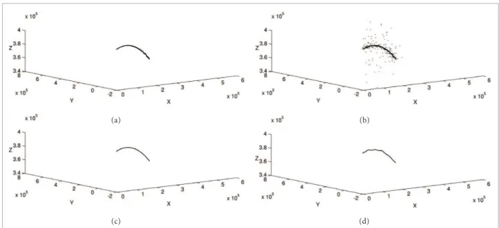
In Fig. 1, the tridimensional plot (a) shows 2,177 reasonably well behaved trajectory data points (with no extreme outliers) obtained from radar tracking of the International Space Station (ISS) while plot (b) shows the result of a 5% artii cial outlier contamination procedure applied to the original data. Plot (c) shows the resulting smoothed curve from LOESS application over the original points from plot (a) while plot (d) shows the distorting ef ects caused by these outliers to the resulting LOESS smoothed curve, using the same smoothing parameters as in plot (c). In this work, all original test datasets were purposely artii cially contaminated for better illustration of outlier ef ects and ef ectiveness of the techniques used in this work.
To overcome the influence of the outliers, a robust version of the LOESS has been referenced in the literature. h e robustii cation consists, basically, in iterative reweighting
processes that involve building robust weights with a specii ed robustness weight function by using current residuals and updating those on each iteration, until the residuals remain unchanged. However, these additional steps add much more computation complexity to the LOESS and dramatically decrease its performance (Cleveland, 1979; Cleveland et al., 1990; Garcia, 2010). In our preliminary tests, robust LOESS was proved unattractive because it took too long to converge and neglected to several extreme outliers.
Smoothing Splines (Penalized Least Squares)
Another popular and established non-parametric regression is smoothing splines, which is based on the optimization of a penalized least squares criterion whose solution is a piecewise polynomial or a spline function (Loader, 2012). h is approach employs i tting a spline with knots at every data point, so it could potentially i t perfectly into data, but the function parameters are estimated by minimizing the usual sum of squares plus a roughness penalty dei ned by the penalized sum of squares criterion (Garcia, 2010). An amount of penalty is imposed according to the magnitude of the tuning parameter (also known as degree of freedom) of the method, so that the lower is the parameter the closer is the data i t, which could lead to a noisy curve, as it follows every detail in data. h e higher is the parameter, the smoother is the solution curve, which could end up in a very poor i t to data.
Figure 1. Inl uence of outliers on LOESS smoothing procedure. (a) Original data; (b) Original data with 5% artii cial outliers contamination; (c) LOESS applied to original data; (d) LOESS applied to outlier contamined data.
(a) (b)
It is a well known fact that the results obtained with smoothing splines are very similar to LOESS results. Moreover, the main drawback of smoothing splines is the proved sensitivity to outliers (Garcia, 2010). hese facts were conirmed in preliminary tests with our trajectory datasets. Generally, even using a higher tuning parameter, the method tends to overit misbehaving data (dispersed and highly-contaminated), always leading to a less smoothed output than the LOESS’ output for the same scenario. Although it is a good, fast and well-referenced method, it proved to be less efective than LOESS when considering our trajectory datasets.
OUTLIER DETECTION
Although there is no single, unanimously accepted or rigid mathematical definition of what an outlier is, there is a consensus on referring to outliers as a statistical term for an observation that is numerically much deviant from the behaviour obser ved in the majority of the data. In statistics, there is a wide and classic discussion regarding the characterisation and categorisation of these unusual observations in outliers, high-leverage points and influential points. However, since this kind of analysis is not the focus of this work, we will not go into the merits of these differentiations.
Outliers are perhaps the simplest and best-known type of data anomaly (Pearson, 2005), highly common in most applied and scientific scenarios involving data collection and analysis. In terms of our trajectography dataset, outliers can be seen as points that disobey the general pattern of smooth variation seen in the data sequence, which represents the flight of an aerospace engine which is bound to the laws of physics.
These data anomalies demand close attention, because they are observations that do not follow the statistical distribution of the bulk of the data, and consequently, may lead to erroneous results regarding statistical analysis (Liu
et al., 2004). The presence of even a few of these anomalies in a large dataset can have a disproportional influence on analytical results (Pearson, 2005) and may cause general distortions, estimation biasing and inflated error rates that could lead to false alarms, improper decision making, faulty conclusions, model misspecification, etc.
In general, outliers may be treated merely as an extreme manifestation of the random variability inherent of the data, hence, they have to be retained and processed in the same
manner as the other observations (ASTM International, 1980), or as a representation of some disorder or unexpected conditions in the system, such as gross measurement, sampling, computing or recording errors, transient malfunctioning, noise, missing data, human errors, etc. In the latter case, the identified implausible values may eventually be rejected, statistically adjusted and/or held for further analysis. Discussion regarding what to do with identified outliers is a common and controversial topic in outlier detection literature, but there is a consensus that outliers should not be simply discarded, since they may carry important (or key) information and insights about the process. After all, “one person’s noise could be another person’s signal”.
Outlier detection has been suggested to detect implausible behaviour points for numerous applications such as business transactions, clinical trials, voting, network intrusion, weather prediction, geographic information systems, chemical data processing, industrial process monitoring, and so forth (Pearson, 2005; Nurunnabi and Nasser, 2008). Although dealing with outliers is an old and well-known problematic, there is no ultimate outlier identification procedure which is able to cover all kinds of outlier scenarios. Even so, since there are different types of outliers emanating from various sources and influencing data analysis in different ways, as well as there is no rigid formalisation of what constitutes an outlier, the identification of these doubtful observations is an arduous and ultimately a matter of interpretation, or at least previous knowledge of the data.
outlier detection: masking and swamping. Masking is the inability of a procedure to detect actual outliers while the swamping is the detection of a legit observation as an outlier. Literature shows that these opposing effects are faced by all outlier identification methods in a complementary fashion: a procedure which performs well with respect to masking is more susceptible to swamping and vice-versa (Pearson, 2005; Pearson, 2011).
Cook’s distance is a general method for assessing the local influence of single data point against least squares regression analysis. The goal of the method is to detect influential points in regression coefficients, but it cannot be considered a conclusive test to detect outliers because it is very prone to both masking and swamping effects (Rancel and Sierra, 2000; Adnan et al., 2003; Nurunnabi and Nasser, 2008).
Other widely known method is the Dixon’s Q for outlier detection, mainly because of its simplicity. It is based on a comparison between the suspect value and its direct or close neighbour with the overall or modified range. A point is flagged as outlier if its calculated Q value exceeds the critical Q-value presented in a static table at the chosen significance level. Although it was originally recommended by ISO for inter-laboratorial tests, this test should be used just once in a dataset to detect a unique outlier, because it is highly prone to masking effects (Massart et al., 1997).
The Grubbs’ test for outliers is a commonly used procedure which replaced Dixon’s Q test on ISO recommendations (Horwitz, 1995). It is suggested in order to detect outliers in a univariate dataset assumed to come from an approximately normally distributed population. The test is based on the difference of the mean of the sample and the farthermost data, considering the standard deviation. Although it has been modified and adapted (Horwitz, 1995; NIST/ SEMATECH, 2012), this procedure still suffer from series of limitations, like the normality assumption, the use of non-robust characterisation tools, such as mean and standard deviation as core statistics, and the inability of reasonably detecting multiple outliers (Zhang et al., 2004; Solak, 2009; NIST/SEMATECH, 2012).
Another popular approach to outlier identiication is the well-known 3σ edit rule, based on the idea that, if data sequence
is assumed to be approximately normally distributed, the probability of observing a point farther than three standard deviations from the mean is only about 0.3% (Pearson, 2002). Despite its historical importance and intuitive appeal, this outlier
detection procedure tends to be inefective in practice. he basic weakness is that the presence of outliers in the dataset can cause substantial errors in both estimated mean and standard deviation in which the procedure is based. It makes outliers harder to point out and, consequently, too few outliers are detected (Pearson, 2005).
From the described so far, it is noticeable that there is the need for a versatile outlier detection procedure, which could work independently from the distribution type assumption, capable of sanely detecting multiple outliers without a process model or assumptions and based on robust (outlier-resistant) statistical tools. he Hampel ilter, regarded as one of the most robust and eicient outlier identiier (Liu et al., 2004), satisies these requirements by running through data a moving window cleaner centred at the current data point, using robust core statistics. A robust adaptation of the 3σ edit rule, named Hampel
identiier, is then applied to this window to characterise each point regarding a local neighbourhood of preceding and subsequent samples, producing the replacement of the data point declared to be an outlier with a more representative value, according to other data points in the immediate vicinity, otherwise the data point is unchanged (Pearson 2005; Pearson, 2011).
The Hampel identifier, base processing of the Hampel filter, consists of replacing the original data location and data standard deviation estimates in the 3-σ edit rule.
The mean is replaced with the median and the standard deviation is substituted with the MAD (Median Absolute Deviation). Because median and MAD are both less sensitive to outliers than the mean and standard deviation, respectively, the Hampel identifier behaves much more effectively than the 3 σ edit rule in a majority of outlier scenarios (Pearson, 2005;
Pearson, 2011). The main drawback of these replacements is that the overall outlier detection procedure becomes more aggressive and, consequently, legit data may be declared as outliers. Then, this identifier is naturally more sensitive to the swamping effect than to masking effects. Davies and Gather (1993) reasonably described in details the overall Hampel functioning, including the employed criteria used in order to evaluate if a sample is an outlier.
The Hampel filter has only two tuning parameters: the half-width K of the window and the threshold parameter t
for t = 0, for which it is reduced to the median filter, since the target sample will always be replaced with the median of the window. In the other extreme, if t is large enough, the target sample will stay unmodified unless the MAD scale estimate is zero. This condition only occurs when a majority of values in the moving window are exactly the same, for example, when processing a coarsely quantised dataset (Pearson, 2005), which is not the case in our experiments.
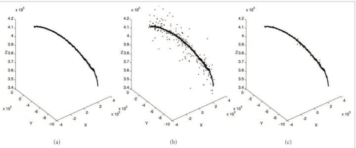
The behaviour of the Hampel filter, applied to our trajectory datasets, was very satisfactory. For example, when the filter was processed over a test trajectory dataset, this procedure was able to detect about 90% of those artificial outliers, which purposely contaminated the original dataset (10% of the total samples). It also pointed out some evident abehant samples within the original data. Figure 2 plots illustrates the Hampel filter response to the previously contaminated ISS trajectory data, using K=3 and t=3. Plot (c) shows that most outlying samples were detected and replaced with the median of their surroundings. This is a good example of small but beneficial distortions introduced by this filter to an outlier contaminated dataset.
RADAR DATA FILTERING
The main interest in this research is to clean up tracking data of aerospace engines collected from a trajectory radar
system, producing as result a smooth and outlier free curve that would afford much more accurate results regarding online and offline analyses. Due to the proven effectiveness and popularity of LOESS and the Hampel filter in their respective fields, they were chosen to integrate our proposal as base statistics.
PROPOSAL
The proposal consists on submitting trajectory radar data to a data filtering system founded on outlier detection/ substitution and smoothing phases. The outlier detection pre-processing phase is borne to the Hampel filter while LOESS takes the charge of the main process of smoothing. It is important to highlight that, for illustration purposes, all original tracking datasets were submitted to an outlier contamination process based mostly in the application of additive Gaussian white noise to some randomly chosen samples, in order to simulate a slight distortion of the signal. These signal distortions could be caused, for example, by adverse weather conditions, malfunctioning of some radar subsystem or channel interferences.
The first approach to address the issue of cleaning radar data is to run both procedures sequentially on offline radar data. This would yield an after flight quality plot of the just tracked aerospace target to radar experts, helping them on reporting clean plots, extracting meaningful trends from radar data, detecting disagreements regarding nominal trajectories, modelling trajectories, etc. The second approach
Figure 2. Hampel ilter work over outlier-contaminated trajectory data. (a) Original data; (b) 10% Outlier contamination e (c) Hampel iltered data.
is supposed to be online and it involves establishing a moving window with parameterized bandwidth to be applied to incoming radar data, producing an on flight outlier-free and smoothed curve, which could be used for an accurate calculation of instant speed and acceleration of the target, determination of a less dispersed area of impact and establish concise extrapolations on the trajectory in case of radar malfunctioning or tracking loss.
IMPLEMENTATION
In these early research phases, it is important to prioritize a proper evaluation of the effectiveness of the methods under study over the achieved performance. After the validation of the effectiveness of the methodology, performance considerations should be taken into account. Given that, it is convenient in study and prototype phases to use numerical computing environments for the sake of simplicity, abstraction and flexibility, despite the well-known performance issues inherent to these environments. Several environments such as Matlab, R and Scilab were used in our experiments since most building blocks used in our approach are already satisfactorily implemented in these numerical environments. The dataset is basically composed by tridimensional Cartesian coordinates converted from azimuth, elevation and distance coordinates of trajectory data generated by the radar during the tracking of a target. As they are obtained from different radar subsystems, they can be considered independent measures. Then, each trajectory coordinate is separately treated as a univariate time series, which is conjoined with the others only for plotting purposes.
The offline approach was implemented in a straight-forward way. It consists on the sequential submission of the target dataset to both Hampel filter and LOESS procedures with predefined parameter values to get as result an outlier-free and smoothed curve which may better reflect the trajectory of the aerospace engine.
The online approach rendered somewhat more work, since a moving window to be applied to the incoming data needs to be established. To ensure the online scenario, a 20 Hz sampling rate to the already existent trajectory datasets is simulated. Thus, a sliding window is established, taken into account a fixed proportion of the full dataset points to set the window size. To step the window through data, it is required to fill a buffer with the latest incoming points. Thus, at each fulfilment of the buffer, the window moves a
step and the overall processing is applied to it. The step size could be the whole window bandwidth or a fixed proportion of it. The overall processing has to be accomplished as fast as data arrives, once the online approach is supposed to support radar analysts’ decisions and derivative processing during the flight of the engine.
RESULTS
EFFECTIVE COMBINATION
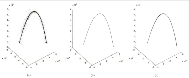
In most tests, the filtering process combining outlier detection and smoothing successfully delivered an outlier-free and smooth curve that, according to radar specialists, does not afront rocket models and nominal trajectories. he results are quite satisfactory as both procedures on which our approach is based performed very well in their actuation fields. The Hampel ilter played an important pre-processing role as the routine preceding the LOESS smoother, especially in scenarios of high contamination. In most tested datasets, Hampel ilter could show an identiication rate exceeding 80% in relation to artiicial outlying data. It was also able to ensure that the most signiicant outliers would not render much interference in local regression. Figure 3 shows a comparative plot set for oline and online iltering approaches. Figure 3 (a) presents a 10% artiicial outlier contamination on a certain rocket trajectory data and Fig. 3 (b) reveals the oline results regarding the application of the iltering processes, using the parameters K=3, t=3 (Hampel ilter) and g=0.5, d=2 (LOESS). A locally quadratic it (d=2) was used in all LOESS tests.
Regarding the smoothing phase, it was observed significant differences between offline and online results. Offline results were quite impressive, since the output curve was indeed smooth, reflecting better the actual trajectory of the target flying engine. On the other hand, the results from the online implementation pointed out that there is a serious trade-off related to the size of the moving window and the effectiveness of the LOESS smoothing procedure.
It happens because LOESS requires a fairly large and densely sampled datasets in order to produce good models. h at is, it needs good empirical information on the local structure of the process in order to perform the local i tting (NIST/SEMATECH, 2012). When the dataset is partitioned in windows that move as data arrives, much less data is delivered to each iteration of the LOESS procedure, making the smoothing process much more local when considering the whole dataset. Besides, as the LOESS procedure is invoked more ot en (at least in each window iteration), a performance drop is also justii able. Substantially increasing the moving window bandwidth is not the solution to this problem, because this would make this online approach gradually closer to the ol ine approach. Since the methods are computationally intensive, limited computational capabilities becomes a crucial barrier in the online approach.
Figure 3 (c ) also shows the results when applying the online method on the contaminated dataset, using the same parameters used on offline experiments (for Hampel filter and LOESS) and a window size w=100 (one hundred samples) for the moving window applied to incoming data. The online method outputs a slightly less smooth curve than the offline results and it is much more computationally intensive.
EXTRAPOLATING FILTERED DATA
Because of the good results after applying the filtering processes, it was expected that any further processing
applied to this smooth and well-behaved data would render better results when compared to the processing of raw radar data. From existing filtered source data, extrapolation could play an important role by completing the missing portion of the signal in a tracking loss scenario or by predicting with better accuracy the impact point of a falling aerospace engine.
To prove this hypothesis, we decided to extrapolate both filtered and unfiltered data using a well known and effective extrapolation method and comparing the results. A proven effective and established method that could fit well to the problem was chosen. A linear predictive strategy using autoregressive modeling was preferred as its attractiveness stems, among others, from the fact that the numerical algorithms involved in the processing are rather simple and it depends on a limited number of parameters which are estimated from the already measured data (De Hoon
et al., 1996). However, this strategy produces coefficients which are not well suited for numerical computation and models which are not always stable. To overcome these constraints, the preferable algorithm to estimate the autoregressive parameters is the Burg’s method, due to its reliability and accuracy on parameter estimates and because the estimated autoregressive model is guaranteed to be stable (De Hoon
et al., 1996).
To sum up very briefly, we used the strategy mentioned above to extrapolate a time series (each of the three
Figure 3. A comparative plot set for ofl ine and online i ltering approaches. (a) Original data with 10% outlier contamination; (b) Ofl ine i ltered curve; (c) Online i lltered curve.
x 105
x 104
8 7
7 6
6 5
5 4
4 3
3 2
2 1
1 0
0 -1
-1 1000
-1000 -2000
-3000 -4000
-5000 -6000
-7000 -8000 0
Base data
Extrapolated data
Start of extrapolation
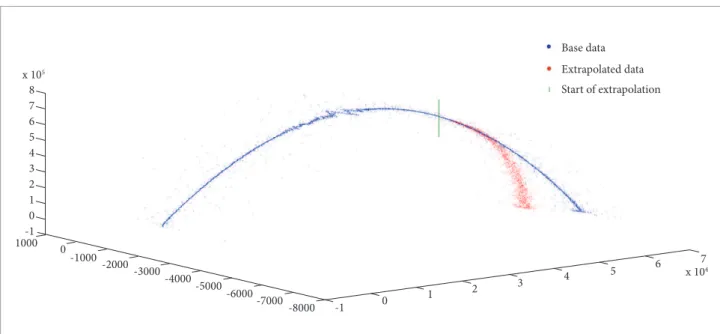
Figure 4. Extrapolation of uniltered radar data.
signal components) by fitting a linear model to the time series, in which each sample is assumed to be a linear combination of previously observed samples. Hence, the predicted samples are the next time samples of the input time segment.
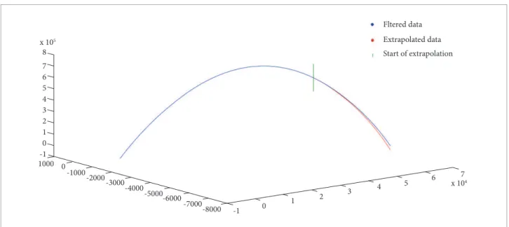
he following igures illustrate the results of applying Burg’s extrapolation over both uniltered and iltered radar data, obtained from the tracking of a certain rocket. Again, for illustration purposes, the base data used in these extrapolation experiments is the original tracking data with 5% of samples artiicially contaminated by outliers. Figure 4 shows a tridimensional plot comparing the entire base data to its extrapolation, starting from the 3501st of a 5820 sample total. A noticeable deviation between
the uniltered samples curve and the extrapolated samples curve can be noted. On the other hand, the tridimensional plot of Fig. 5 clearly shows that the deviation between the iltered data and its extrapolation is much lower.
DISCUSSION AND FUTURE WORK
This work represents just a primer approach to trajectory radar data cleaning, supported by a long-standing demand brought about by radar specialists. Preliminary results were considered quite satisfactory, mainly regarding the
offline processing. The problem of outlying samples was reasonably surpassed and data analysts can rely on a smoother and more representative curve for subsequent analysis. Online processing demands more work regarding the optimal strategy on processing incoming radar data as the efficient use of a stepping moving window limits the amount of data delivered to smoothing processes and, consequently, degrades the quality of the smoothed curve. Besides, for effectiveness and performance reasons, it is essential to implement online processing methods in low-level programming languages, since the online approach needs several iterations of already costly processes, and the processed results should be instantly available.
As for what to be done with the filtered data, the possibilities are vast. It was shown that, from a smooth and well behaved trajectory curve, extrapolation strategies could be readily applied in case of radar malfunctioning and target loss. Also, it is possible to adjust parametric models to the curve which can propitiate accurate speed and acceleration calculations on specific points of the trajectory. These approaches could also be used in a scenario where it is needed to determine precisely the area of impact of a tracked flying engine.
x 105
x 104
8
7
7 6
6 5
5 4
4 3
3 2
2 1
1 0
0 -1
-1 1000
-1000 -2000
-3000 -4000
-5000 -6000
-7000 -8000 0
Fltered data
Extrapolated data
Start of extrapolation
Figure 5. Extrapolation of iltered radar data.
parameter tuning algorithm to select the best parameters
given the trajectory shape and quality of radar data. Also, the independent trajectory coordinates problematic is likely to be a good candidate for parallel or distributed
processing approach in order to speed up the overall process, especially for the online filtering process.
A lot of validation work has to be done in order to
verify if the output model really befits the actual trajectory of a tacked aerospace engine. This validation work may consider past tracking datasets, analytic physical
REFERENCES
Adnan, R., Mohamad, M.N. and Setan, H., 2003, “Multiple Outliers Detection Procedures in Linear Regression”, Matematika, Vol. 19, No 1, pp. 29-45.
ASTM International, 1980, “Standard Practice for Dealing with Outlying Observations”, Active Standard E-178-08.
Cleveland, R.B., Cleveland, W.S., McRae, J.E. and Terpenning I., 1990, “STL: A seasonal-trend decomposition procedure based on LOESS”, Journal of Oficial Statistics, Vol. 6, No 1, pp.3–73.
Cleveland, W.S. and Devlin, S.J., 1988, “Locally Weighted Regression: An Approach to Regression Analysis by Local Fitting”, Journal of the American Statistical Association, Vol. 83, No 403, pp. 596-610.
Cleveland, W.S. and Loader, C.L., 1996, “Smoothing by Local Regression: Principles and Methods”, Statistical Theory and Computational Aspects of Smoothing, pp. 10-49, Haerdle and M. G. Schimek, Springer, NY.
Cleveland, W.S., 1979, “Robust Locally Weighted Regression and Smoothing Scatterplots”, Journal of the American Statistical Association, Vol. 74, No 368, pp. 829–836. doi:10.1080/0162 1459.1979.10481038.
Cohen, R. A., 1999, “An Introduction to PROC LOESS for Local Regression”, Proceedings of the 24th SAS Users Group International Conference, Paper 273.
Davies, L. and Gather, U., 1993, “The identification of multiple outliers”, Journal of the American Statistical Association, Vol. 88, No 423, pp. 782–792. doi:10.1080/01621459.19 93.10476339.
De Hoon, M.J.L., van der Hagen, T.H.J.J., Schoonewelle, H. and van Dam, H., 1996, “Why Yule-Walker should not be used for autoregressive modeling”, Annals of Nuclear Energy, Vol. 23, No 15, pp. 1219–1228. doi:10.1016/0306-4549(95)00126-3.
analyses data and nominal trajectory behavior data for a specific engine.
ACKNOWLEDGMENT
Garcia, D, 2010, “Robust smoothing of gridded data in one and higher dimensions with missing values”, Computational Statistics & Data Analysis, Vol. 54, No 4, pp. 1167-1178. doi:10.1016/ j.csda.2009.09.020.
Horwitz, W., 1995, “Protocol for the Design, Conduct and Interpretation of Method-performance Studies”, Pure & Applied Chemistry, Vol. 67, No 2, pp. 331-343. doi:10.1351/pac199567020331.
Lee, J., Han, J. and Li, X., 2008, “Trajectory Outlier Detection: A Partition-and-Detect Framework”, Proceedings of the IEEE 24th International Conference on Data Engineering (ICDE ‘08), pp. 140-149.
Liu, H., Shah, S. and Jiang, W., 2004, “On-line outlier detection and data cleaning”, Computers & Chemical Engineering, Vol. 28, Issue 9, pp. 1635–1647. doi:10.1016/j.compchemeng.2004.01.009.
Loader, C., 2012, “Smoothing: Local Regression Techniques”, Handbook of Computational Statistics, Ch. 20, pp. 571-596. doi:10.1007/978-3-642-21551-3_20.
Massart, D. L., Vandeginste, B.G.M., Buydens, L.M.C., De Jong, S., Lewi, P.J. and Smeyers-Verbek, J., 1997, “Handbook of Chemometrics and Qualimetrics: Part A”, Data Handling in Science and Technology, Elsevier Science, Vol. 20A.
NIST/SEMATECH, 2012,“e-Handbook of Statistical Methods”, Retrieved in May 27, 2013, from http://www.itl.nist.gov/div898/handbook/.
Nurunnabi, A.A.M. and Nasser, M., 2008, “Multiple Outliers Detection: Application To Research & Development Spending and Productivity Growth”, BRAC University Journal, Vol. V, No 2, pp. 31-39.
Pearson, R. K., 2002, “Outliers in process modeling and identiication”, IEEE Transactions on Control Systems Technology, Vol. 10, No 1, pp. 55-63. doi:10.1109/87.974338.
Pearson, R.K., 2005, “Mining Imperfect Data: Dealing with Contamination and Incomplete Records”, SIAM.
Pearson, R.K., 2011, “Exploring Data in Engineering, the Sciences, and Medicine”, Oxford University Press, 2011.
Rancel, M.M.S. and Sierra, M.A.G., 2000, “Procedures for the Identiication of Multiple Inluential Observations Using Local Inluence”, The Indian Journal of Statistics (Sankhy ), Series A, Vol. 62, No 1, pp. 135-143.
Simonoff, J.S., 1998, “Smoothing Methods in Statistics”, 2nd edition, Springer.
Solak, M.K., 2009, “Detection of Multiple Outliers in Univariate Data Sets”, Schering-Plough Research Institute, Summit, NJ, paper SP06-2009, Retrieved in May 27, 2013, from http://www. lexjansen.com/pharmasug/2009/sp/SP06.pdf.
Wilson, D.I., 2006, “The Black Art of Smoothing”, Electrical and Automation Technology, June/July Issue.