The effect of support springs in ends welded gap
hollow YT-joint
Abstract
This paper presents an analysis on the effect of support springs in an ends circular hollow sections welded into a YT joint. The overall behavior and failure of the joint were characterized under axial compression of the lap brace. Two joint failure modes were identified: chord wall plastification (Mode A) and cross-sectional chord buckling (Mode F) in the region below the lap brace. The system was modeled with and without support springs using the numerical finite element program Ansys. Model results were compared with experimental data in terms of principal stress in the joint in-tersection. The finite element model without support springs proved to be more accurate than that with support springs. Keywords
support springs, hollow structures, YT joints, numerical analysis, experimental analysis.
R. F. Vieira∗
and J. A. V. Requena
State University of Campinas, Faculty of Civil Engineering, Architecture and Urbanism, Department of Structural Engineering, SP – Brazil
Received 14 Sep 2010; In revised form 8 Apr 2011
∗Author email: [email protected]
1 INTRODUCTION
One of the reasons that steel structures are used more frequently in buildings nowadays is that their manufacturing process presents several economic advantages. In this context, the increasing worldwide demand for hollow structural steel sections must be pointed out; these structural sections have provided many buildings with an elegant and modern look. Thus, one of the factors that determine the cost of steel structures is the manufacturing of standardized hollow sections.
The most common hollow sections have square (SHS-Square Hollow Sections), rectangular (RHS-Rectangular Hollow Sections), or circular cros sections (CHS-Circular Hollow Sections). They are made of highly resistant steel, with a yield stress of around 350 MPa. One of the companies that manufacture this material in Brazil is Vallourec & Mannesmann Tubes, or V&M do Brasil S.A. (formerly Mannesmann S.A.). It was founded in 1953 at the request of the Brazilian government, to meet the growing demand of their domestic oil industry.
NOMENCLATURE
Ai cross sectional area of memberi (i=0,1,2,3);
E modulus of elasticity;
Et modulus of elasticity tangent;
M0 bending moment in the chord member;
Ni axial force applied to memberi(i=0,1,2,3);
N∗
i joint design resistance expressed in terms of axial load in member i;
N0P pre-stressing axial force on the chord;
W0 elastic section modulus of memberi(i=0,1,2,3);
di external diameter of circular hollow section for member i(i=0,1,2,3);
e nodding eccentricity for a connection;
fy yield stress;
fyi yield stress of memberi (i=0,1,2,3);
f0P pre-stress in chord;
f(n′
) function which incorporates the chord pre-stress in the joint resistance equation;
g gap between the bracings members of a K, N or KT joint, at the face of the chord;
g′
gap divided by chord wall thickness;
n′ f0P
fy0
= N0P
A0⋅fy0 +
M0
W0⋅fy0
ti thickness of hollow section member i(i=0,1,2,3);
β diameter ratio between bracing on chord;
β =d1
d0,
d1
b0,
bi
b0 T, Y and X
β =d1+d2 2⋅d0 ,
d1+d2 2⋅b0 ,
b1+b2+h1+h2
4⋅b0 K and N
γ ratio of the chord’s half diameter to its thickness;
ν poisson’s ratio
θ included angle between bracing member i(i=0,1,2,3)and the chord;
ϵ maximum specific proportionality strain;
f stress;
flp maximum proportionality stress;
fr maximum resistance stress;
f1 principal stress 1;
f2 principal stress 2;
fy yield strength;
the Finite Element Method [1, 2, 4], and analytical work aimed at developing mathematical expressions of the joint strength [6].
employed the Ansys program to model the hollow joints as an assembly of “shell” elements. Numerical finite element models using Ansys, with and without support springs, were compared with the experimental data in terms of principal stress in the joint intersection.
A great deal of experimental research has been done on welded hollow sections to explore the various possible failure modes in such systems. The results depend on the joint type, load conditions, and many other geometrical parameters. There are several formulations describing the failure modes; some derive from theoretical studies, while others are merely empirical models.
2 CALCULATION OF CONNECTION RESISTANCE
The YT joint prototype design uses the methodology presented by Wardenier et al. [11] and Packer and Henderson [7].
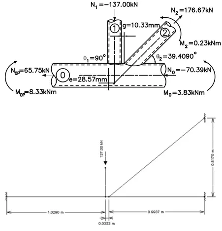
The Fig. 1 shows forces general scheme using as a limit the maximum capacity of the vertical brace member of the YT joint and the bending moment due the eccentricity was not considered [9, 10].
Figure 1 Forces general scheme of YT joint.
in the YT joint. The nominal physical proprieties yield stress (fy) are equal 250 MPa.
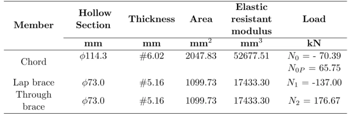
Table 1 Physical and geometrical characteristics.
Member
Hollow
Section Thickness Area
Elastic resistant modulus
Load
mm mm mm2
mm3
kN
Chord ϕ114.3 #6.02 2047.83 52677.51 N0= - 70.39
N0P = 65.75
Lap brace ϕ73.0 #5.16 1099.73 17433.30 N1 = -137.00
Through
brace ϕ73.0 #5.16 1099.73 17433.30 N2 = 176.67
2.1 Validity limits
The YT joint meets all geometrical requirements described in the aforementioned references.
2.2 Calculations
A) YT joint parametersThe YT joint parameters are given by Eq. (1) through Eq. (5):
β= d1+d2 2⋅d0
; (1)
g′
= g
t0
; (2)
The stress on the chord, f0P, depends most critically on the compressing stress.
n′
= f0P
fy0
= N0P
A0⋅fy0
+ M0
W0⋅fy0
; (3)
f (n′
)=1.0+0.3⋅n′ − 0.3⋅n′2 ≤ 1 ; (4)
f (γ, g′
)=γ0.2⋅(1+ 0.024⋅γ
1.2
1+exp(0.5⋅g′−1.33)); (5)
B) Plastic failure of the chord face (Mode A)Vertical lap brace:
N∗ 1 =
fy0⋅t 2 0
senθ1 (
1.8+10.2⋅d1
d0)
⋅f (γ, g′) ⋅ f (n′); (6)
N∗ 2 =N
∗ 1 ⋅(
senθ1
senθ2)
; (7)
C) Punching shear failure of the chord face (Mode B) Vertical lap brace and diagonal
through brace are both given by Eq. (8):
N∗
i =
fy0⋅t0⋅π⋅di √
3 ⋅ (
1+senθi 2⋅sen2θi)
; (8)
D) YT Joint Resistance The joint resistance is the lowest value obtained in items (B) and (C) above.
Vertical lap brace:
N1
N∗ 1
<1; (9)
Diagonal through brace:
N2
N∗ 2
<1; (10)
Table 2 presents the results of the calculation.
Table 2 Results of the calculation procedure.
Joint parameters Acronym Calculation
Relation between diameters β 0.64
Relation between diameter and thickness γ 9.49
n′
=stress/fy (compression) n′ -0.14
Function of prestress on chord f(n′
) 0.95
Resistance plastic failure of the chord face (Mode A) N∗
1(P l) 137.40 kN
Resistance punching shear failure of the chord face (Mode B) N∗
1(P u) 199.27 kN
Lap brace use N1/N
∗
1 1.0
Resistance plastic failure of the chord face (Mode A) N∗
2(P l) 216.42 kN
Resistance punching shear failure of the chord face (Mode B) N∗
2(P u) 404.16 kN
Through brace use N2/N
∗
2 0.82
3 EXPERIMENTAL PROGRAM
3.1 YT Joint Prototypes
The dimensions of the prototypes are shown in Fig. 2. The prototypes are fixed by four screws at each end. They were loaded axially at the top of the lap brace.
Figure 2 YT joint prototype (mm).
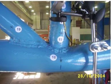
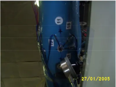
3.2 Instrumentation for tests
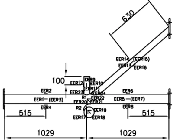
In EXPERIMENTS I, II and III, sixteen 5mm electrical resistance KFG-5-120-C1-11 exten-someters were used. Their positions are marked EER1 to EER16 in Fig. 3.
The EERs were placed on the prototype to measure longitudinal strain, drawing on the work of Fung et al [5]. In EXPERIMENT III, 2 rosette gauges and 2 individual extensometers were added (for a total of 24 EERs). Rosette 1 was composed of EER20, EER21 and EER22; rosette 2 was composed of EER17, EER18 and EER19. EER23 and EER24 were placed at the bases of the lap brace and through brace respectively.
Figure 3 Positioning of the extensometers on the YT joint prototype.
Figure 4 Positioning of the TDs on the YT joint prototype.
3.3 Experimental results
The testing methodology used was defined in three stages, as shown below:
• Stage I- Before starting the test, the prototype was subjected to a cycle of 10 loading of approximately 20% of the estimated collapse loading for the connection, to minimize friction and check the torque of the screws. Based on pre-test the loading was estimated at 50kN. This level of loading is within the elastic limit of the material. The force was applied in small increments and then it was done downloading.
• Stage II - During the test the speed of the actuator load was kept as slow and steady as possible for both the case of loading and for unloading. The step load was previously set depending on the stage supposed to loading. At each step of loading, when the pre established loading was reached, expected time to stabilize the transducers and then did the reading.
• Stage III- The prototype was loaded to the ultimate state, where the prototype did not offer more resistance, even after he reached the break. Then the prototype was unloaded.
Figure 5 Overall strain of the prototype for Experiment III.
Figure 7 Failure Mode F: local buckling of the chord face.
The results presented by extensometers in each Experiments I, II and III are similar, are representing the state of tension expected for each region and thus show that the tests were equivalent.
The results of the last loading for each of the tests are shown in Table 3.
Table 3 Last loading to Experiments I, II and III. Experiments Last loading
(kN)
Experiment I 240,0
Experiment II 358,6 Experiment III 316,4
Two failure modes were observed: plastic failure of the chord face (Mode A) and local buckling of the chord walls (Mode F).
4 ANALYSIS OF FINITE ELEMENTS
Two numerical models were created in Ansys, one using a bilinear stress-strain diagram (BISO – Bilinear Isotropic Hardening) and the other a multilinear (piecewise linear) diagram (MISO – Multilinear Isotropic Hardening). Their results were compared to the experimental tests [9, 10].
of diameter 114.3mm [9, 10].
The contour conditions were simulated in Ansys through displacement restrictions. Force was applied in an increasing way, that is, at unit load pitches.
Fig. 8 and Fig. 9 show the stress-strain diagrams of test bodies selected for the numerical analysis. The multilinear model is represented by 26 points (crossed circles), and the bilinear model by two straight lines (triangles).
Figure 8 Experimental, bilinear and multilinear stress-strain diagrams used for test body cp1b, from the through brace and lap brace (φ73mm).
Table 4 shows data used to represent the material properties of test bodies cp1b and cp2b in the numerical model. Note that the bilinear stress-strain diagram always runs from the origin to the first stress peak (f), then from this point to the maximum stress (fr) of the material.
Table 4 Data used to represent the bilinear stress-strain diagram with the Ansys software (BISO).
Test Body fy f fr E Et
MPa MPa MPa MPa MPa
cp1b(ϕ73mm) 326.0 331.1 486.9 189114.6 856.5 cp2b(ϕ114.3mm) 322.6 322.6 473.6 227390.8 840.6
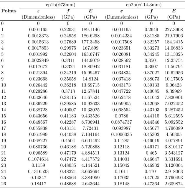
The 26 points to represent the multilinear stress-strain diagram is shown by Table 5. The Poisson’s ratio was obtained by compression test tube used. The value obtained was
ν = 0.3.
The SHELL element was considered most appropriate to represent hollow structures. Specifically, the SHELL181 element was used to generate a mesh for the hollow sections, Fig. 10. The SHELL63 element was used for fixation plates. Table 6 shows their characteristics.
Table 5 Data used to represent the multilinear stress-strain diagram with the Ansys software (MISO).
Points
cp1b(ϕ73mm) cp2b(ϕ114,3mm)
ε f E ε f E
(Dimensionless) (GPa) (GPa) (Dimensionless) (GPa) (GPa)
0 0 0 0 0 0 0
1 0.001165 0.22031 189.1146 0.001165 0.2649 227.3908
2 0.0013373 0.24958 186.6298 0.0014234 0.31285 219.7906
3 0.0015613 0.27689 177.3458 0.0017508 0.32257 184.2415
4 0.0017853 0.29975 167.899 0.023651 0.33273 14.06833
5 0.001992 0.32604 163.6747 0.026081 0.34245 13.13025
6 0.0022849 0.3311 144.9079 0.028562 0.3501 12.25754
7 0.017672 0.3324 18.80942 0.031181 0.3607 11.56794
8 0.021394 0.34219 15.99467 0.034834 0.37027 10.62956
9 0.023668 0.35058 14.8124 0.037418 0.38073 10.17505
10 0.026442 0.36218 13.69715 0.043173 0.39133 9.06423
11 0.029286 0.3713 12.67841 0.047722 0.40085 8.39969
12 0.032646 0.38115 11.67524 0.052478 0.41042 7.820801
13 0.036229 0.39585 10.92633 0.059905 0.42068 7.022452
14 0.038728 0.40007 10.33025 0.068554 0.43103 6.287452
15 0.043656 0.41183 9.433526 0.0786 0.44115 5.612595
16 0.048567 0.42287 8.706941 0.0874737 0.44546 5.092552
17 0.055838 0.43131 7.72431 0.093987 0.45077 4.796089
18 0.061989 0.44038 7.104164 0.1006035 0.45302 4.50305
19 0.068227 0.4504 6.601492 0.11285 0.46019 4.077891
20 0.080736 0.46188 5.720868 0.12118 0.46171 3.810117
21 0.096589 0.47179 4.884511 0.13124 0.465 3.543127
22 0.1074614 0.47472 4.417572 0.14001 0.46647 3.331691
23 0.1159 0.48035 4.144521 0.15042 0.46932 3.120064
24 0.1316533 0.48221 3.662694 0.1611 0.4701 2.918063
25 0.14347 0.48564 3.384959 0.17035 0.47025 2.760493
Elements
Nr of nodes per
element
Degrees of freedom
Special features
SHELL 63 4 6 Elastic Large
deflection Little strain
SHELL 181 4 6 Plastic Large
deflection Large strain
5 COMPARISON BETWEEN EXPERIMENTAL TEST RESULTS AND NUMERICAL MODEL RESULTS
The experimental tests and numerical models can be compared on the basis of strains obtained by the extensometers [9, 10].
For the rosettes, comparisons between theory and experiment can be made between the principal stresses. Principal stress is the maximum tension that occurs in the place where was positioned the rosettes considered a critical region of the connection.
Fig. 11 show the principal stresses f1 measured at rosette 1 in Experiment III and the
numerical models.
Figure 11 Principal stressf1 measured at rosette 1 in Experiment III and the numerical models.
The principal stresses f1 of the two numerical models were in good agreement with those
6 THE EFFECT OF SUPPORT SPRINGS
Numerical modeling for the simulation of the connection between the end plates of the pro-totype in the test frame requires special care. Numerical modeling this connection may be performed using the effect of springs. The springs serve to give less rigidly to connect. It will be represented in this work for two situations: Case A, with support springs, and Case B, without support springs.
6.1 Case A: with support springs
For determining the value of the spring constant “Ksprings” the test frame was analyzed with unitary loading in two positions. A for the displacement toward of the plate ends of the prototype the chord and other through brace. In the first measurement, loading was applied toward the plate ends of the prototype (the chord); in the second, loading was applied toward the plate ends of the prototype (through the brace). The spring constant is given by Eq. (11).
Ksprings=
F
δ (11)
Where F is the unitary loading and δ is the displacement.
The test frane modeled in SAP2000 to obtain the value of displacement is shown in Fig. 12.
Figure 12 Test frame modeled in SAP2000.
For the through-brace loading, the value of the displacementδ1was found to be 0.02868mm
and Ksprings1 = 34.87kN/mm. For the chord loading, the displacement δ2 was found to be
0.01673mm and Ksprings2 = 59.77kN/mm.
6.2 Case B: without support springs
7 COMPARISON BETWEEN EXPERIMENTAL TEST RESULTS AND NUMERICAL MODEL RESULTS
Fig. 13 shows the principal stresses f1obtained by numerical models analyzing Case A (with
support springs), and Case B (without support springs), along with data collected with rosette 1 in Experiment III.
Figure 13 Comparison between numerical models Case A (with support springs) and Case B (without support springs). Data collected with rosette 1 in Experiment III are also shown..
Table 7 shows the relative error between the principal stressesf1obtained by the numerical
models and the experimental data.
Table 7 Relative error between the principal stressesf1 obtained by numerical models (Cases A and B) and
the rosette 1 data in Experiment III.
Load (kN) Experiment Case A Case B Error % Case A
Error % Case B f1 (Mpa) f1 (Mpa) f1 (Mpa)
50.0 90.4 76.0 92.7 15.9 2.5
75.0 136.6 114.3 139.4 16.3 2.0
100.2 183.5 153.0 186.6 16.6 1.7
125.0 233.1 192.9 236.1 17.3 1.3
151.0 311.5 241.8 297.3 22.4 4.6
160.4 346.6 263.4 319.7 24.0 7.8
170.0 376.6 286.5 345.9 23.9 8.2
8 CONCLUSIONS
Comparisons between theoretical and experimental values of the principal stresses can be made for the rosettes. The experimental tests and numerical analysis were consistent in indicating that the most critical region of the joint is its intersection, where the greatest stress concen-tration is found. At this spot there was plasticization.
For each of the hollow sections, the yield stress fy can be obtained by finding the average of the stresses provided during the traction test. The average yield stress of the chord was 330 MPa. The yield load of the YT joint was whatever load induced the yield stress in at least one section.
The yield load measured by rosette 1 in the experiments may not be the yield load of the YT joint, however, because the yield may have occurred at some other point. Still, it must be very close as numerical models identify this area as having the greatest stress concentration. With numerical modeling, it is possible to obtain the yield load at the location corresponding to rosette 1. It also provides the yield load of the finite element model, which can be compared to the yield load of the real YT joint.
Table 7 shows the relative error between the principal stresses f1 obtained by the numerical models Case A and Case B and those measured by rosette 1 in Experiment III. The error between the Case A and experimental values is around 25%, which is quite high. The Case B error is only around 10%, a much better agreement with the experimental data. The finite element model without support springs thus proved to be more accurate than the finite element model with support springs.
AcknowledgementsThe authors are grateful for the support from UNICAMP, from Vallourec & Mannesmann Tubes (V&M do Brasil).
References
[1] E.M. Dexter and M. M. K. Lee. Static strength of axially loaded tubular K-joint. I: Behaviour.Journal of Structural
Engineering, 125(2):194–201, 1999.
[2] E.M. Dexter and M. M. K. Lee. Static strength of axially loaded tubular K-joint. II: Ultimate capacity. Journal of
Structural Engineering, 125(2):202–210, 1999.
[3] EUROCODE 3. Design of steel structures. part1.1: General rules and rules for buildings. Technical Report Annex K. Env 1993-1-1, 1992.
[4] T. C. Fung, C. K. Soh, and W. M. Gho. Ultimate capacity of completely overlapped tubular joints – II. Behavioural
study. Journal of Constructional Steel Research, 57(8):881–906, 2001.
[5] T. C. Fung, C. K. Soh, W. M. Gho, and F. Qin. Ultimate capacity of completely overlapped tubular joints – I. An
experimental investigation.Journal of Constructional Steel Research, 57(8):855–880, 2001.
[6] Y. Kurobane, Y. Makino, and K. Ochi. Ultimate resistance of unstiffened tubular joints. Journal of Structural
Engineering, 110(2):385–400, 1984.
[7] J. A. Packer and J. E. Henderson. Hollow structural section joints and trusses: a design guide. Canadian Institute
of Steel Construction, Ontario, 2nd edition, 1997.
[8] J. A. Packer, J. Wardenier, Y. Kurobane, D. Dutta, and N. Yeomans. Design guide for rectangular hollow section
[9] R.F. Vieira, J.A.V. Requena, A.M.S. Freitas, and V.F. Arcaro. Numerical and experimental analysis of yield loads
in welded gap hollow YT-joint. Latin American Journal of Solids and Structures, 6(4):363–383, 2009.
[10] R.F. Vieira, J.A.V. Requena, A.M.S. Freitas, and V.F. Arcaro. Behavior analysis of bar gaps in welded YT-joints
for rolled-steel circular hollow sections. Latin American Journal of Solids and Structures, 7(4):369–389, 2010.
[11] J. Wardenier, Y. Kurobane, J. A. Packer, D. Dutta, and N. Yeomans.Design guide for circular hollow section (CHS)