Analytical study on the vibration frequencies of tapered beams
Abstract
A vast amount of published work can be found in the field of beam vibrations dealing with analytical and numerical tech-niques. This paper deals with analysis of the nonlinear free vibrations of beams. The problem considered represents the governing equation of the nonlinear, large amplitude free vi-brations of tapered beams. A new implementation of the an-cient Chinese method called the Max-Min Approach (MMA) and Homotopy Perturbation Method (HPM) are presented to obtain natural frequency and corresponding displacement of tapered beams. The effect of vibration amplitude on the non-linear frequency is discussed. In the end to illustrate the effectiveness and convenience of the MMA and HPM, the obtained results are compared with the exact ones and shown in graphs and in tables. Those approaches are very effective and simple and with only one iteration leads to high accuracy of the solutions. It is predicted that those methods can be found wide application in engineering problems, as indicated in this paper.
Keywords
large amplitude free vibrations, analytical solution, tapered beam, Homotopy Perturbation Method (HPM), Max-Min Approach (MMA).
Mahmoud Bayat∗,a, Iman Pakara and Mahdi Bayata
Department of Civil Engineering, Shirvan Branch, Islamic Azad University, Shirvan, Iran
Received 23 Nov 2010; In revised form 21 Dec 2010
∗Author email: [email protected]
1 INTRODUCTION
Galerkin, harmonic balance method and simple harmonic oscillations. Singh et al [32] later studied the large-amplitude vibration problem of unsymmetrically laminated beams based on classical, first-order and higher-order formulations by using the numerical integration technique introduced earlier by Singh et al [31]. Qaisi [25] used an analytical method for determining the vibration modes of geometrically nonlinear beams under various edge conditions. Rehfield [27] proposed an approximate method for nonlinear vibration problems with material nonlin-ear effects for various boundary conditions. Sathyamoorthy [28] developed the work on finite element method for nonlinear beams under static and dynamic loads and classical methods for the analysis of beams with material, geometric and other types of nonlinearities. Raju
et al [26] studied the large amplitude vibration problem of beams and plates using Rayleigh-Ritz method by incorporating the inplane deformation as well as inertia, which were absent in the earlier studies, and also by retaining the equivalent linearization function. Klein [13] used finite element approach and Rayleigh-Ritz for analyzing the vibration of the tapered beams. A dynamic discretization technique was applied to calculate the natural frequencies of a non-rotating double tapered beam based on both the Euler-Bernoulli and Timoshenko Beam Theories by Downs [5]. Sato [29] improved the Ritz method to study a linearly tapered beam with ends restrained elastically against rotation and subjected to an axial force. Lau [14] used the exact method for studying on the free vibration of tapered beam with end mass. The Green’s function method in Laplace transform domain was used to study the vibration of general elastically restrained tapered beams by Lee et al [15] for obtaining the approximate fundamental solution by using a number of stepped beams to represent the tapered beam. Junioret al [21] proposed Galerkin Method and the Askey-Wiener scheme as solutions of the stochastic beam bending problem. Oni and Awodola considered [3] the Dynamic response under a moving load of an elastically supported non-prismatic Bernoulli-Euler beam on vari-able elastic foundation. Boukhalfa and Hadjoui [4] analyzed the free vibration of an embarked rotating composite shaft using the hp- version of the FEM.
The main objectives of this study are to use analytical methods for analyzing the free vibration of the tapered beams. Finding an exact analytical solution for nonlinear equations is extremely difficult. Therefore, many analytical and numerical approaches have been inves-tigated. The most useful methods for solving nonlinear equations are perturbation methods. They are not valid for strongly nonlinear equations and they have many shortcomings. Many new techniques have appeared in the open literature to overcome the shortcomings of tra-ditional analytical methods such as Variational Iteration [10, 18], Parameter-Expansion [19], Energy Balance [2, 12, 16, 22], Variational Approach [33], Iteration Perturbation [23], the Im-proved Amplitude-frequency Formulation [35] and differential transformation [20], etc. In this study, which is an extension of the authors’ previous work [1], Max-Min Approach (MMA) and Homotopy Perturbation Method (HPM) were developed by J.H. He [8, 9] and investigated in different works [17, 30, 34], which have the following advantages, over above-mentioned methods:
2. In MMA and HPM, just one iteration leads us to high accuracy of solutions which are valid for a wide range of vibration amplitudes.
The Max-Min Approach (MMA) and Homotopy Perturbation Method (HPM) are used to find analytical solutions for this problem with the nonlinear governing differential equation. It is shown that the solutions are quickly convergent and their components can be simply calculated. The results of the MMA and HPM are compared with the exact one, it can be observed that MMA and HPM are accurate and require smaller computational effort. An excellent accuracy of the MMA and HPM results indicates that those methods can be used for problems in which the strong nonlinearities are taken into account.
2 TAPERED BEAM FORMULATION
In dimensionless form, the governing differential equation corresponding to fundamental vi-bration mode of a tapered beam is given by Goorman [7] and the schematic of a tapered beam represented by Fig. 1:
(d2u
dt2)+ε1(u 2
(d2u dt2)+u(
du dt)
2
)+u+ε2u 3
=0 (1)
Where u is displacement and ε1 and ε2 are arbitrary constants. Subject to the following
initial conditions:
u(0)=A, du(0)
dt =0 (2)
Figure 1 Schematic representation of a tapered beam.
3 OVERVIEW OF HE’S MAX-MIN APPROACH METHOD
We consider a generalized nonlinear oscillator in the form;
u′′
+u f(u)=0, u(0)=A, u′(0)=0, (3)
u(t)=Acos(ωt), (4)
Where ω the unknown frequency to be further is determined. Observe that the square of frequency, ω2
, is never less than that in the solution
u1(t)=Acos(
√
fmint), (5)
Of the following linear oscillator
u′′
+u fmin=0, u(0)=A, u
′
(0)=0, (6)
Where fmin is the minimum value of the functionf(u).
In addition, ω2
never exceeds the square of frequency of the solution
u1(t)=Acos(
√
fmint), (7)
Of the following oscillator
u′′
+u fmin=0, u(0)=A, u
′
(0)=0, (8)
Where fmax is the maximum value of the functionf(u).
Hence, it follows that
fmin
1 <ω
2
<fmax
1 . (9)
According to the Chentian interpolation [8, 11], we obtain
ω2= m fmin+n fmax
m+n , (10)
Or
ω2= fmin+kfmax 1+k
, (11)
Wheremandnare weighting factors,k=n/m. So the solution of Eq. (3) can be expressed as
u(t)=Acos √
fmin+kfmax
1+k t, (12)
The value of kcan be approximately determined by various approximate methods [22, 23, 33]. Among others, hereby we use the residual method [11]. Substituting Eq. (12) into Eq. (3) results in the following residual:
Where ω=√fmin+kfmax
1+k
If, by chance, Eq. (12) is the exact solution, then R(t;k) is vanishing completely. Since our approach is only an approximation to the exact solution, we set
∫0T
R(t;k)cos √
fmin+kfmax
1+k tdt=0, (14)
Where T =2π/ω. Solving the above equation, we can easily obtain
k= fmax−fmin 1−√A
π∫ π
0 cos
2x.f(Acosx)dx
. (15)
Substituting the above equation into Eq. (12), we obtain the approximate solution of Eq. (3).
4 OVERVIEW OF HOMOTOPY PERTURBATION METHOD (HPM)
To explain the basic idea of the HPM for solving nonlinear differential equations, one may consider the following nonlinear differential equation:
A(u)−f(r)=0 r∈Ω (16)
That is subjected to the following boundary condition:
B(u,∂u
∂t)=0 r∈Γ (17)
WhereAis a general differential operator,Ba boundary operator,f(r)is a known analytical function, Γ is the boundary of the solution domain(Ω), and∂u/∂tdenotes differentiation along the outwards normal to Γ. Generally, the operatorA may be divided into two parts: a linear part Land a nonlinear part N. Therefore, Eq. (16) may be rewritten as follows:
L(x)+N(x)−f(r)=0 r∈Ω (18)
In cases where the nonlinear Eq. (16) includes no small parameter, one may construct the following homotopy equation
H(ν, p)=(1−p) [L(ν)−L(x0)]+p[A(ν)−f(r)]=0 (19)
Where
ν(r, p)∶Ω×[0,1]→R (20)
In Eq. (19), p ∈[0,1] is an embedding parameter and u0 is the first approximation that
ν=ν0+pν1+p 2
ν2+ ⋯ (21)
The homotopy parameter p is also used to expand the square of the unknown angular
frequency ω as follows:
ω0=ω 2
−pω1−p 2
ω2− ⋯ (22)
Or
ω2=ω0+pω1+p 2
ω2+ ⋯ (23)
whereω0is the coefficient ofu(r)in Eq. (16) and should be substituted by the right hand side
of Eq. (23). Besides, ωi(i=1,2, . . .)are arbitrary parameters that have to be determined. The best approximations for the solution and the angular frequencyω are
u=lim p→1
ν=ν0+ν1+ν2+ ⋯ (24)
ω2=ω0+ω1+ω2+ ⋯ (25)
when Eq. (19) corresponds to Eq. (16) and Eq. (24) becomes the approximate solution of Eq. (16).
5 APPLICATIONS 5.1 Solution using MMA
We can re-write Eq. (1) in the following form
(ddt2u2)+
⎛ ⎝
1+ε1(dudt) 2
+ε2u 2
1+ε1u2
⎞
⎠u=0 (26)
We choose a trial-function in the form
u=Acos(ωt) (27)
Where ω the frequency to be is determined.
By using the trial-function, the maximum and minimum values of ω2
will be:
ωmin=
1+ε1A2ω2
1 , ωmax=
1+ε2A2
1+ε1A2
. (28)
So we can write:
1+ε1A 2
ω2
1 <ω
2
< 1+ε2A
2
1+ε1A2
(29)
ω2= m.(1+ε1A
2
ω2
+ε2A2)+n.(1+ε1A2ω2)
m+n =1+ε1A
2
ω2+kε2A 2
(30)
Where m and n are weighting factors, k = n/m+n. Therefore the frequency can be
approximated as:
ω= √
1+kε2A2
1−ε1A2
(31)
Its approximate solution reads
u=Acos √
1+kε2A2
1−ε1A2
t (32)
In view of the approximate solution, Eq. (32), we re-write Eq.(??) in the form
d2
u dt2 +(
1+kε2A2
1−ε1A2 )
u=(d
2
u
dt2)+ε1(u 2
(ddt2u2)+u(
du dt)
2
)+u+ε2u 3
+Ψ (33)
Ψ=(1+kε2A
2
1−ε1A2 )
u−ε1u 2
(ddt2u2)−ε1u(
du dt)
2
−u−ε2u 3
(34)
Substituting the trial function into Eq. (34) , and using Fourier expansion series, it is obvious that:
Ψ=(1+kε2A
2
1−ε1A2 ) (
Acosωt)−(2ω2ε1A 2
cos2(ωt)−ε1A 2
ω2−1−ε2A 2
cos2(ωt))Acos(ωt)
= ∞ ∑ n=0
b2n+1cos[(2n+1)ωt]=b1cos(ωt)+b3cos(3ωt)+...≈b1cos(ωt)
(35)
For avoiding secular term we set b1=0
∫ T/
4
0 ((
1+kε2A2
1−ε1A2 )
−(2ω2ε1A 2
cos2(ωt)−ε1A 2
ω2−1−ε2A 2
cos2(ωt)))Acos(ωt)dt=0 (36)
Where T =2π/ω. Solving the above equation, we can easily obtain
k=−(ε1ω
2 −ε21A
2
ω2
+3ε1−2ε2+2ε2A 2
ε1)
3ε2
(37)
Substituting Eq. (37) into Eq. (32), yields
ω= √
(3+ε1A2) (2ε2A2+3)
(3+ε1A2)
According to Eqs. (38) and (38), we can obtain the following approximate solution:
u(t)=Acos⎛ ⎝
√
(3+ε1A2) (2ε2A2+3)
(3+ε1A2)
t⎞
⎠ (39)
5.2 Solution using HPM
Eq. (1) can be rewritten as the following form:
(ddt2u2)+u+p.[ε1u 2
(ddt2u2)+ε1u(
du dt)
2 +ε2u
3
]=0, p∈[0,1]. (40)
To explain the analytical solution, the solution u and the square of the unknown angular frequency ω are expanded as follows:
u=u0+pu1+p 2
u2+ ⋯ (41)
1=ω2−pω1−p 2
ω2− ⋯ (42)
Substituting Eqs.(41) and (42) into Eq. (40) and equating the terms with identical powers of p, the following set of linear differential equations is obtained:
p0∶ (d
2
u0
dt2 )+ω 2
u0=0 (43)
p1∶ u¨1+ω 2
u1=ε1u0(
du0
dt )
2 +ε1(
d2
u0
dt2 )u 2
0−ω1u0+ε2u 3
0, (44)
Solving Eq. (43) gives: u0=Acosωt. Substitutingu0 into Eq. (44), yield:
p1∶ (d
2
u1
dt2 )+ω 2
u1=ε1ω 2
A3cos(ωt)sin2(ωt)−ε1ω 2
A3cos3(ωt)
+ω1Acos(ωt)+ε2A 3
cos3(ωt)
(45)
For achieving the secular term, we use Fourier expansion series as follows:
Φ(ω, t)=ε1ω 2
A3cos(ωt)sin2
(ωt)−ε1ω 2
A3cos3
(ωt)+ω1Acos(ωt)+ε2A 3
cos3
(ωt)
= ∞ ∑ n=0
b2n+1cos[(2n+1)ωt]
=b1cos(ωt)+b3cos(3ωt)+ ⋯
≈(∫ π/2
0 Φ(
ω, t)d(ωt))cos(ωt)
=[(Aω1+
1 3A
3
ε1ω 2
−2
3A
3
ε2)]cos(ωt)
Substituting Eq. (46) into Eq. (45) yields:
p1∶ u¨1+ω 2
u1=[(Aω1+
1 3A
3
ε1ω 2
−2
3A
3
ε2)]cos(ωt)+
∞ ∑ n=0
b2n+1cos[(2n+1)ωt] (47)
Avoiding secular term, gives:
ω1=−
1 3A
2
(ε1ω 2
−2ε2) (48)
From Eq. (42) and setting p=1, we have:
1=ω2−ω1 (49)
Comparing Eqs. (48) and (49), we can obtain:
ω2=−1
3A
2
(ε1ω 2
−2ε2)+1 (50)
Solving Eq. (50), gives:
ωHP M = √
(3+ε1A2) (2ε2A2+3)
(3+ε1A2)
(51)
6 RESULTS AND DISCUSSIONS
Comparisons with the analytical methods and the exact one are presented to illustrate and verify the accuracy of the Max-Min Approach (MMA) and Homotopy Perturbation Method (HPM). The exact frequencyωe for a dynamic system governed by Eq. (1) can be derived, as
shown in Eq. (52), as follows:
ωExact=2π/4√2A∫ π/2
0
√
1+ε1A2cos2tsint
√ A2(1
−cos2t) (ε2A2cos2t+ε2A2+2)
dt (52)
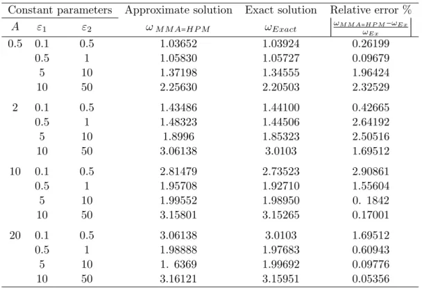
To demonstrate the accuracy of the MMA and HPM , the procedures explained in previous sections are applied to obtain natural frequency and corresponding displacement of tapered beams. A comparison of obtained results from the Max-Min Approach and Homotopy pertur-bation method and the exact one is tabulated in Table 1 for different parameters A, ε1 and
ε2.
From Table 1, the relative error of the analytical approaches is 2.90861% for the first-order analytical approximations, for A = 10, ε1 = 0.1 and ε2 = 0.5. To further illustrate
Table 1 Comparison of frequency corresponding to various parameters of system.
Constant parameters Approximate solution Exact solution Relative error %
A ε1 ε2 ωM M A=HP M ωExact ∣
ωM M A=H P M−ωEx
ωEx ∣
0.5 0.1 0.5 1.03652 1.03924 0.26199
0.5 1 1.05830 1.05727 0.09679
5 10 1.37198 1.34555 1.96424
10 50 2.25630 2.20503 2.32529
2 0.1 0.5 1.43486 1.44100 0.42665
0.5 1 1.48323 1.44506 2.64192
5 10 1.8996 1.85323 2.50516
10 50 3.06138 3.0103 1.69512
10 0.1 0.5 2.81479 2.73523 2.90861
0.5 1 1.95708 1.92710 1.55604
5 10 1.99552 1.98950 0. 1842
10 50 3.15801 3.15265 0.17001
20 0.1 0.5 3.06138 3.0103 1.69512
0.5 1 1.98888 1.97683 0.60943
5 10 1. 6369 1.99692 0.09776
10 50 3.16121 3.15951 0.05356
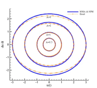
Figure 2 Comparison of analytical solutions ofu(t)based ontwith the exact solution forε1=0.1,ε2=0.5,A=
2.
Figure 3 Comparison of analytical solutions ofu(t)based ontwith the exact solution forε1=0.1,ε2=0.5,A=
approaches with the exact one for different values of amplitude, and shows the phase-space curves ( ˙u(t) versus u(t) curve) of the Eqs. (51, 38) for amplitudes, u(0)=0.5,1,2 and 3. It can be observed that the phase-space curve generated from MMA and HPM are close to that of the exact curve. The phase plot shows the behavior of the oscillator whenε1=0.5,ε2=0.1.
It is periodic with a center at (0, 0). This situation also occurs in the unforced, undamped cubic Duffing oscillators.
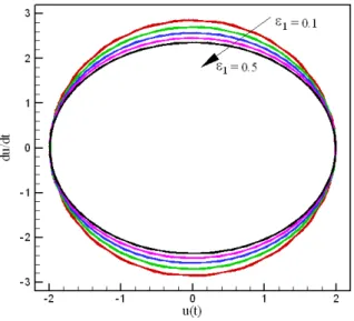
Figure 4 Comparison of analytical solutions of du/dt based on u(t) with the exact solution forε1 = 0.5, ε2=0.1.
Figure 5 Comparison of frequency corre-sponding to various parameters of amplitude (A) andε1=1.
Figure 7 Phase plane, forA=2,ε2=0.5.
The effect of small parameters ε1 and ε2 on the frequency corresponding to various
pa-rameters of amplitude (A) has been studied in Figs. 5 and 6 for ε1 and ε2. Also, the phase
plane for this problem obtained from MMA and HPM has been shown in Fig. 7. It is evident that MMA and HPM show excellent agreement with the numerical solution using the exact solution and quickly convergent and valid for a wide range of vibration amplitudes and initial conditions. The accuracy of the results shows that the MMA and HPM can be potentiality used for the analysis of strongly nonlinear oscillation problems accurately.
7 CONCLUSIONS
References
[1] M. Bayat, M. Shahidi, A. Barari, and G. Domairry. The approximate analysis of nonlinear behavior of structure under harmonic loading. International Journal of the Physical Sciences, 5(7):1074–1080, 2010.
[2] M. Bayat, M. Shahidi, A. Barari, and G. Domairry. Analytical evaluation of the nonlinear vibration of coupled oscillator systems.Zeitschrift f¨ur Naturforschung A - A Journal of Physical Sciences, 66(1-2):67–74, 2011.
[3] Abdelkrim Boukhalfa and Abdelhamid Hadjoui. Free vibration analysis of an embarked rotating composite shaft using the hp- version of the FEM. Latin American Journal of Solids and Structures, 7:105–141, 2010.
[4] Claudio Roberto Avila da Silva Junior, Andre Teolo Beck, and Edison da Rosa. Solution of the stochastic beam bend-ing problem by Galerkin method and the Askey-Wiener scheme. Latin American Journal of Solids and Structures, 6:51–72, 2009.
[5] B. Downs. Transverse vibrations of cantilever beam having unequal breadth and depth tapers. ASME J. Appl. Mech., 44:737–742, 1977.
[6] D.A. Evensen. Nonlinear vibrations of beams with various boundary conditions. AIAA J., 6:370–372, 1968.
[7] D.J. Goorman. Free vibrations of beams and shafts. Appl. Mech., ASME, 18:135–139, 1975.
[8] J. H. He. Max-Min approach to nonlinear oscillators. International Journal of Nonlinear Sciences and Numerical Simulation, 9(2):207–210, 2008.
[9] J.H. He. Homotopy perturbation technique.Computer Methods in Applied Mechanics and Engineering, 178:257–262, 1999.
[10] J.H. He. Variational iteration method-a kind of non-linear analytical technique: Some examples. International Journal of Non-Linear Mechanics, 34(4):699–708, 1999.
[11] J.H. He and H. Tang. Rebuild of king fang 40 bc musical scales by He’s inequality.Appl Mech Comput, 168(2):909– 914, 2005.
[12] N. Jamshidi and D.D. Ganji. Application of energy balance method and variational iteration method to an oscillation of a mass attached to a stretched elastic wire.Current Applied Physics, 10(A202):484–486, 2010.
[13] L. Klein. Transverse vibrations of non-uniform beam.J. Sound Vibr., 37:491–505, 1974.
[14] J.H. Lau. Vibration frequencies of tapered bars with end mass. ASME J. Appl. Mech., 51:179–181, 1984.
[15] S.Y. Lee and Y.H. Kuo. Exact solution for the analysis of general elastically restrained non-uniform beams. ASME J. Appl. Mech., 59:205–212, 1992.
[16] I. Mehdipour, D.D. Ganji, and M. Mozaffari. Application of the energy balance method to nonlinear vibrating equations. Current Applied Physics, 10(1):104–112, 2010.
[17] Mo Miansari, Me Miansari, A. Barari, and G. Domairry. Analysis of blasius equation for flat-plate flow with infinite boundary value.International Journal for Computational Methods in Engineering Science and Mechanics, 11(2):79– 84, 2010.
[18] S. T. Mohyud-Din. Modified variational iteration method for integro-differential equations and coupled systems. Z. Naturforsch, 65a:277–285, 2010.
[19] S. T. Mohyud-Din, M. A. Noor, and K. I. Noor. Parameter-expansion techniques for strongly nonlinear oscillators.
Int. J. Nonlin. Sci. Num. Sim., 10(5):581–583, 2009.
[20] M. Omidvar, A. Barari, M. Momeni, and D.D. Ganji. New class of solutions for water infiltration problems in unsaturated soils.Geomechanics and Geoengineering: An International Journal, 5(2):127–135, 2010.
[21] S. T. Oni and T. O. Awodola. Dynamic response under a moving load of an elastically supported non-prismatic Bernoulli-Euler beam on variable elastic foundation.Latin American Journal of Solids and Structures, 7:3–20, 2010.
[22] T. Ozis and A. Yildirim. Determination of the frequency-amplitude relation for a duffing-harmonic oscillator by the energy balance method. Computers and Mathematics with Applications, 54:1184–1187, 2007.
[24] S.R.R. Pillai and B.N. Rao. On nonlinear free vibrations of simply supported uniform beams.J.Sound Vib., 159:527– 531, 1992.
[25] M.I. Qaisi. Application of the harmonic balance principle to the nonlinear free vibration of beams. Appl. Acoust., 40:141–151, 1993.
[26] I.S. Raju, G.V. Rao, and K.K. Raju. Effect of longitudinal or inplane deformation and inertia on the large amplitude flexural vibrations of slender beams and thin plates.J. Sound Vib., 49:415–422, 1976.
[27] L.W.A. Rehfield. Simple, approximate method for analysing nonlinear free vibrations of elastic structures. J. Appl. Mech., ASME, 42:509–511, 1975.
[28] M. Sathyamoorthy. Nonlinear analysis of beams, Part II: Finite-element methods. Shock Vib. Dig., 14:7–18, 1982.
[29] K. Sato. Transverse vibrations of linearly tapered beams with ends restrained elastically against rotation subjected to axial force. Int. J. Mech. Sci., 22:109–115, 1980.
[30] M. Shaban, D.D. Ganji, and M.M. Alipour. Nonlinear fluctuation, frequency and stability analyses in free vibration of circular sector oscillation systems.Current Applied Physics, 10(5):1267–1285, 2010.
[31] G. Singh, G.V. Rao, and N.G.R. Iyengar. Reinvestigation of large amplitude free vibrations of beams using finite elements. J. Sound Vib., 143:351–355, 1990.
[32] G. Singh, G.V. Rao, and N.G.R. Iyengar. Analysis of the nonlinear vibrations of unsymmetrically laminated composite beams.AIAA J., 29:1727–1735, 1991.
[33] L. Xu. Variational approach to solitons of nonlinear dispersive K(m,n) equations. Chaos, Solitons & Fractals, 37:137–143, 2008.
[34] El¸cin Yusufo˘glu. An improvement to homotopy perturbation method for solving system of linear equations. Com-puters & Mathematics with Applications, 58(11-12):2231–2235, 2009.