A refined shear deformation theory for flexure of thick beams
Abstract
A Hyperbolic Shear Deformation Theory (HPSDT) taking into account transverse shear deformation effects, is used for the static flexure analysis of thick isotropic beams. The dis-placement field of the theory contains two variables. The hyperbolic sine function is used in the displacement field in terms of thickness coordinate to represent shear deformation. The transverse shear stress can be obtained directly from the use of constitutive relations, satisfying the shear stress-free boundary conditions at top and bottom of the beam. Hence, the theory obviates the need of shear correction factor. Gov-erning differential equations and boundary conditions of the theory are obtained using the principle of virtual work. Gen-eral solutions of thick isotropic simply supported, cantilever and fixed beams subjected to uniformly distributed and con-centrated loads are obtained. Expressions for transverse dis-placement of beams are obtained and contribution due to shear deformation to the maximum transverse displacement is investigated. The results of the present theory are com-pared with those of other refined shear deformation theories of beam to verify the accuracy of the theory.
Keywords
hyperbolic shear deformation theory, static flexure, general solution of beams, shear contribution factor.
Yuwaraj M. Ghugal∗ and Rajneesh Sharma
Department of Applied Mechanics, Govern-ment College of Engineering, Aurangabad-431005, Maharashtra State – India
Received 20 Dec 2010; In revised form 21 Dec 2010
∗Author email: [email protected]
1 INTRODUCTION
The Bernoulli-Euler elementary theory of bending (ETB) of beam disregards the effect of the shear deformation. The theory is suitable for slender beams and is not suitable for thick or deep beams since it is based on the assumption that the transverse normal to the neutral axis remains so during bending and after bending, implying that the transverse shear strain is zero. Since the theory neglects the transverse shear deformation, it underestimates deflections and overestimates the natural frequencies in case of thick beams, where shear deformation effects are significant.
NOMENCLATURE
A Cross sectional area of beam;
b Width of beam in y direction;
E, G, µ Elastic constants of the material;
E Young’s modulus;
G Shear modulus;
h Thickness of beam;
I Moment of inertia of cross section of beam;
L Span of the beam;
q Intensity of uniformly distributed transverse load;
u Axial displacement inx direction;
w Transverse displacement in z direction;
x, y, z Rectangular Cartesian coordinates;
µ Poisson’s ratio of the beam material;
σx Axial stress inx direction;
τxz Transverse shear stress inzxplane;
φ Unknown function associated with the shear slope.
ABBREVIATIONS
ETB Elementary Theory of Beam-bending FSDT First-order Shear Deformation Theory HSDT Higher-order Shear Deformation Theory TSDT Trigonometric Shear Deformation Theory PSDT Parabolic Shear Deformation Theory HPSDT Hyperbolic Shear Deformation Theory UDL Uniformly distributed load
that the effect of transverse shear is much greater than that of rotatory inertia on the response of transverse vibration of prismatic bars. In this theory transverse shear strain distribution is assumed to be constant through the beam thickness and thus requires shear correction factor to appropriately represent the strain energy of deformation. Cowper [4] has given refined expression for the shear correction factor for different cross-sections of the beam.
analyses of shear deformable uniform rectangular beams.
The theories based on trigonometric and hyperbolic functions to represent the shear de-formation effects through the thickness is the another class of refined theories. Vlasov and Leont’ev [18] and Stein [13] developed refined shear deformation theories for thick beams in-cluding sinusoidal function in terms of thickness coordinate in the displacement field. However, with these theories shear stress free boundary conditions are not satisfied at top and bottom surfaces of the beam. This discrepancy is removed by Ghugal and Shimpi [7] and developed a variationally consistent refined trigonometric shear deformation theory for flexure and free vibration of thick isotropic beams. Ghugal and Nakhate [5] obtained the general bending so-lutions for thick beams using variationally consistent refined trigonometric shear deformation theory. Ghugal and Sharma [6] developed the variationally consistent hyperbolic shear defor-mation theory for flexural analysis of thick beams and obtained the displacements, stresses and fundamental frequencies of flexural mode and thickness shear modes from free vibration of simply supported beams.
In this paper, a variationally consistent hyperbolic shear deformation theory previously developed by Ghugal and Sharma [6] for thick beams is used to obtain the general bending solutions for thick isotropic beams. The theory is applied to uniform isotropic solid beams of rectangular cross-section for static flexure with various boundary and loading conditions. The results are compared with those of elementary, refined and exact beam theories available in the literature to verify the credibility of the present shear deformation theory.
2 THEORETICAL FORMULATION
The variationally correct forms of differential equations and boundary conditions, based on the assumed displacement field are obtained using the principle of virtual work. The beam under consideration occupies the following region:
0≤x≤L; −b/2≤y≤b/2; −h/2≤z≤h/2
where x, y, z are Cartesian coordinates, L is the length, b is the width and h is the total depth of beam. The beam is subjected to transverse load of intensity q(x) per unit length of the beam. The beam can have any meaningful boundary conditions.
2.1 The displacement field
The displacement field of the present beam theory is of the form [6]
u(x, z) = −zdw
dx +[zcosh(
1
2)−hsinh(
z
h)]ϕ(x) (1)
w(x, z)=w(x) (2)
Here u and w are the axial and transverse displacements of the beam center line in the x
the elementary theory of beam bending (ETB) due to Bernoulli-Euler which is linear through the thickness of the beam the second term in the bracket is the displacement due to transverse shear deformation, which is assumed to be hyperbolic sine function in terms of thickness coordinate, which is non-linear in nature through the thickness of beam. The hyperbolic sine function is assigned according to the shearing stress distribution through the thickness of the beam. Theϕ(x)is an unknown function to be determined and is associated with the rotation of the cross-section of the beam at neutral axis.
Normal strain: εx =
∂u ∂x=−z
d2
w
dx2 +[zcosh( 1
2)−hsinh(
z h)]
dϕ
dx (3)
Shear strains: γxz=
∂u ∂z +
dw
dx =[cosh(
1
2)−cosh(
z
h)]ϕ (4)
Stresses
One dimensional constitutive laws are used to obtain normal bending and transverse shear stresses. These stresses are given by
σx=Eεx, τxz=Gγxz (5)
where E and G are the elastic constants of beam material.
2.2 Governing equations and boundary conditions
Using the expressions (3) through (5) for strains and stresses and dynamic version of principle of virtual work, variationally consistent governing differential equations and boundary conditions for the beam under consideration are obtained. The principle of virtual work when applied to the beam leads to
b∫
x=L x=0 ∫
z=h/2
z=−h/2(σ
xδεx+τxzδγxz)dxdz−∫ x=L x=0 qδwdx
=0 (6)
where the symbol δ denotes the variational operator. Employing Green’s theorem in Eqn. (6) successively, we obtain the coupled Euler-Lagrange equations which are the governing differen-tial equations of the beam and the associated boundary conditions of the beam. The governing differential equations obtained are as follows:
EId
4
w
dx4 −EIA0
d3
ϕ
dx3 =q (7)
EIA0
d3
w
dx3 −EIB0
d2
ϕ
dx2 +GAC0ϕ=0 (8) where A0, B0 and C0 are the constants as given in Appendix and the associated boundary conditions obtained are as follows:
Either EId
3
w
dx3 −EIA0
d2
ϕ
Either EId
2
w
dx2 −EIA0
dϕ
dx =0 or dw
dx is prescribed (10)
Either EIA0
d2
w
dx2 −EIB0
dϕ
dx =0 orφis prescribed (11)
Thus the variationally consistent governing differential equations and the associated bound-ary conditions are obtained. The static flexural behavior of beam is given by the solution of these equations and simultaneous satisfaction of the associated boundary conditions.
2.3 The general solution for the static flexure of beam
Using the governing equations (7) and (8) for static flexure of beam, the general solution for
w(x) and φ(x) can be obtained. By integrating and rearranging the first governing equation (Eqn. 7) one can get following equation
d3
w dx3 −A0
d2
ϕ dx2 =
Q(x)
EI (12)
where Q(x) is the generalized shear force for the beam under consideration and it is given by
Q(x)=∫ q dx+C1. The second governing equation (Eqn. 8) can be written as
d3
w dx3 −
A0
B0
d2
ϕ
dx2 +βϕ=0 (13)
Using Eqn. (12) and Eqn. (13), a single differential equation in terms ofφcan be obtained as follows.
d2
ϕ dx2 −λ
2
ϕ= Q(x)
αEI (14)
where the constant α,β and λ used in Eqn. (13) and Eqn. (14) are given in Appendix. The general solution of above Eqn. (14) is given by:
ϕ(x)=C2coshλx+C3sinhλx−
Q(x)
βEI (15)
The general solution for transverse displacement (w) can be obtained by substituting the expression forϕ(x) in Eqn. (13) and integrating thrice with respect tox. The solution is
EIw(x)=∫ ∫ ∫ ∫ qdxdxdxdx+C1x
3
6 +
A0EI
λ (C2sinhλx+C3coshλx)
+C4
x2
2 +C5x+C6
(16)
3 ILLUSTRATIVE EXAMPLES
3.1 Example 1: Simply supported beam with uniformly distributed load q
A simply supported beam with rectangular cross section (b× h) is subjected to uniformly distributed load q over the span L at surface z = −h/2 acting in the downward z direction.
The origin of beam is taken at left end support i.e. at x = 0. The boundary conditions
associated with simply supported beam are as follows.
EId
3
w dx3 =EI
d2ϕ dx2 =
dw
dx =ϕ=0 atx= L
2 and (17)
EId
2
w dx2 =EI
dϕ
dx =w=0 atx=0, L (18)
The boundary condition, φ = 0 at x = L/2 is used from the condition of symmetry of
deformation, in which the middle cross section of the beam must remain plane without warping (see Timoshenko [15]). Applying appropriate boundary conditions from (19) and (20) in general solutions of the beam the final expressions for φ(x) and w(x) are obtained as follows:
ϕ(x)= qL
2βEI [1−2 x L+
2
λL
sinh(λx−λL/2)
cosh(λL/2) ] (19)
w(x)= qL
4
24EI ( x4
L4−2
x3
L3+
x L)+
3 5 qL2 GA [ x L− x2
L2 − 2
(λL)2(1−
cosh(λx−λL/2)
cosh(λL/2) )] (20)
The maximum transverse displacement at x=L/2 obtained from Eqn. (20) is
w(L/2)= 5qL
4
384EI [1+1.92(1+µ) h2
L2] (21)
3.2 Example 2: Simply supported beam with central concentrated load P
A simply supported beam with rectangular cross section (b×h ) subjected to concentrated load P at mid spani.e. at x=L/2 at surface z=−h/2. The origin beam is taken at left end
support i.e. atx=0. The boundary conditions associated with simply supported beam with
a concentrated load are given as:
EIdw
dx =ϕ=0atx= L
2 and EI
d2
w dx2 =EI
dϕ
dx =w=0atx=0, L (22)
From the condition of symmetry, the middle cross-section of the beam must remain normal and plane, hence shear rotation, φ = 0 at x=L/2 [15]. Using these boundary conditions, in
the region (0=x =L/2) of beam, the general expressions forφ(x) and w(x) are obtained as
follow:
ϕ(x)= P
2βEI [1 −
cosh(λx)
w(x)= P L
3
48EI (3 x L−4
x3
L3)+ 3 5 P L GA( x L− sinhλx
λLcosh(λL/2)) (24)
The maximum transverse displacement at x=L/2 obtained from Eqn. (24) is
w(L/2)= P L
3
48EI [1+2.4(1+µ) h2
L2] (25)
3.3 Example 3: Cantilever beam with uniformly distributed load q
A cantilever beam with rectangular cross section (b×h) is subjected to uniformly distributed load q at surface z=−h/2 acting in the z direction. The origin of beam is taken at free end i.e. at x=0 and it is fixed or clamped at x =L. The boundary conditions associated with
cantilever beam are as given:
EId
3
w dx3 =EI
d2
ϕ dx2 =EI
d2
w dx2 =EI
dϕ
dx =0 atx=0 and dw
dx =ϕ=w=0 atx=L (26)
Using these boundary conditions the general expressions for φ(x) and w(x) are obtained from the general solution as follows:
ϕ(x)= qL βEI [
coshλx
coshλL−
sinhλ(L−x)
λLcoshλL − x
L] (27)
w(x)= qL
4
24EI ( x4 L4 −4
x L+3)+
3 5
qL2 GA[1−
x2 L2−
2(sinhλL−sinhλx)
λLcoshλL +
2 coshλ(L−x)
(λL)2coshλL] (28)
The maximum transverse displacement at free end (x=0) obtained from Eqn. (28) is
w(0)= qL
4
8EI [1+0.8(1+µ) h2
L2] (29)
3.4 Example 4: Cantilever beam with concentrated load P at free end
A cantilever beam with rectangular cross section (b×h) is subjected to concentrated load P at free endi.e. atx=Lat surfacez=−h/2 acting in thez direction. The origin of the beam
is taken at fixed end i.e. at x=0. The boundary conditions associated with cantilever beam
are as given:
EId
2
w dx2 =EI
dϕ
dx =0 atx=Land dw
Using these boundary conditions in general solution of the beam, the general expressions forφ(x) andw(x) are obtained as follows:
φ(x)= P
βEI (sinhλx−coshλx+1) (31)
w(x)= P L
3
6EI (3 x2
L2 −
x3
L3)+ 6 5 P L GA( x L+
coshλx−sinhλx−1
λL ) (32)
The maximum transverse displacement at free end (x=L) obtained from Eqn. (32) is
w(L)= P L
3
3EI [1+0.6(1+µ) h2
L2] (33)
3.5 Example 5: Fixed-fixed (Clamped-clamped) beam with uniformly distributed load q
A fixed-fixed beam with rectangular cross section (b×h) is subjected to uniformly distributed load q at surfacez=−h/2. The origin of the beam is taken at left end fixed/clamped support i.e. x=0. The boundary conditions associated with this beam are as follows:
EId
3
w dx3 =EI
d2
ϕ dx2 =EI
dw
dx =ϕ=0 atx= L
2;
φ=w=EIdw
dx =0 atx=0, Land d2
w dx2 =
dφ dx =
qL2
12EI atx=0 (34)
Using the appropriate boundary conditions, from the set given by Eqn. (34), in general solution of the beam, the general expressions for φ(x) and w(x) are obtained as follows:
ϕ(x)= qL
2βEI [
sinhλ(L/2−x)
sinh(λL/2) −(1−2
x
L)] (35)
w(x)= qL
4
24EI ( x4
L4−2
x3
L3+
x2
L2)+ 3 5 qL2 GA[ x L− x2
L2−
(cosh(λL/2)−coshλ(L/2−x))
λLsinh(λL/2) ] (36)
The maximum transverse displacement at center of the beam (x = L/2) obtained from
Eqn. (36) is
w(L/2)= qL
4
384EI [1+9.6(1+µ) h2
3.6 Example 6: Fixed-fixed beam with central concentrated load P
A fixed-fixed beam with rectangular cross section (b×h) is subjected to concentrated load P at mid span at surface z =−h/2. The origin of the beam is taken at left end fixed/clamped
support i.e. x=0. The boundary conditions associated with this beam are as follows:
EIdw
dx =φ=0atx=0, L
2;w=0 atx=0 and
d2w dx2 =
dφ dx =−
P L
8EI atx=0 (38)
Using these boundary conditions, in the region (0=x=L/2) of beam, the general
expres-sions for φ(x) and w(x) are obtained as follow:
ϕ(x)= P
2βEI (1+sinhλx−coshλx−
sinhλx
sinh(λL/2)) (39)
w(x)= P L
3
48EI (3 x2 L2 −4
x3 L3)+
3 5
P L GA(
x L +
coshλx−sinhλx−1
λL ) (40)
The maximum transverse displacement at center of the beam (x=L/2) obtained from
Eqn. (40) is
w(L/2)= P L
3
192EI [1+9.6(1+µ) h2
L2] (41)
While obtaining the expressions for maximum transverse displacement (deflection) in the above examples it is observed that the quantity λL is very large and therefore tanhλL≃ 1,
1/λL≃ 1/ (λL)2 ≃0 and sinhλL≃coshλL. For problems of practical interest this is a very
good approximation.
4 RESULTS
In expressions of maximum transverse displacement the first term in the bracket is the dis-placement contribution according to the classical Bernoulli-Euler beam theory and the second term represents the effect of transverse shear deformation. These expressions can be written in the generalized form as follows:
w=wC[1+wS(1+µ) (
h L)
2
] (42)
In the above equationwcis the transverse displacement according to the classical
Bernoulli-Euler beam theory andws is the proportionality constant due to transverse shear deformation
effect. In Tables 1 through 3 the values ofws for different beam problems are compared with
Table 1 Values of proportionality constant (ws) for simply supported beams.
Source Model Uniform Load Concentrated
Load
Present HPSDT 1.92 2.4
Timoshenko [14] FSDT 1.92 2.4
Levinson [11] HSDT 1.92 —
Bhimaraddi and Chandrashekhara [2] PSDT 1.92 —
Ghugal and Nakhate [5] TSDT 1.92 2.4
Timoshenko and Goodier [16] Exact 1.93846 —
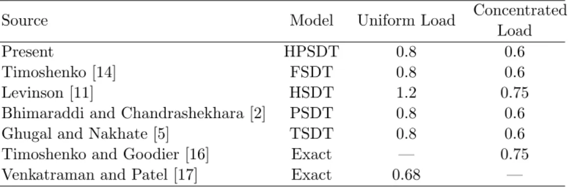
Table 2 Values of proportionality constant (ws) for cantilever beams.
Source Model Uniform Load Concentrated
Load
Present HPSDT 0.8 0.6
Timoshenko [14] FSDT 0.8 0.6
Levinson [11] HSDT 1.2 0.75
Bhimaraddi and Chandrashekhara [2] PSDT 0.8 0.6
Ghugal and Nakhate [5] TSDT 0.8 0.6
Timoshenko and Goodier [16] Exact — 0.75
Venkatraman and Patel [17] Exact 0.68 —
Table 3 Values of proportionality constant (ws) for fixed-fixed beams.
Source Model Uniform Load Concentrated
Load
Present HPSDT 9.6 9.6
Timoshenko [14] FSDT 9.6 9.6
Levinson [11] HSDT 12.0 —
Bhimaraddi and Chandrashekhara [2] PSDT 9.6 —
Ghugal and Nakhate [5] TSDT 9.6 9.6
The numerical results shown in Table 1 for simply supported beam with uniform load and concentrated load indicate that the results of proportionality constant (ws) due to shear
than those obtained by present theory and other refined theories as shown in Tables 2 and 3. However, for cantilever beam with concentrated load Levinson’s theory gives the exact value of this constant (see Table 2). In case of beam with both the ends fixed, it is observed that the constant of proportionality due to shear deformation is independent of loading conditions.
5 CONCLUSIONS
In this paper a hyperbolic shear deformation theory has been used to obtain the bending solutions for thick homogeneous, isotropic, statically determinate and indeterminate beams. General solutions for the transverse displacement and rotation are presented for transversely loaded beams with various end conditions. Expressions for maximum transverse displacements are deduced from the general solutions of the thick beams. The effect of transverse shear deformation on the bending solutions of thick beams can be readily observed from the analytical expressions presented for the transverse displacement. The values of transverse displacement contribution (ws) due to transverse shear deformation effect obtained by present theory are
found to be identical to those of first order shear deformation theory of Timoshenko with the shear correction factor equal to 5/6. The present theory requires no shear correction factor. The accuracy of present theory is verified by comparing the results of other refined theories and the exact theory.
References
[1] M. H. Baluch, A. K. Azad, and M. A. Khidir. Technical theory of beams with normal strain.J. Engg. Mech., ASCE, 110(8):1233–1237, 1984.
[2] A. Bhimaraddi and K. Chandrashekhara. Observations on higher order beam theory. J. Aerospace Engineering, ASCE, 6(4):408–413, 1993.
[3] W. B. Bickford. A consistent higher order beam theory. Dev. in Theoretical and Applied Mechanics, SECTAM, 11:137–150, 1982.
[4] G. R. Cowper. The shear coefficients in Timoshenko beam theory. J. Applied Mechanics, ASME, 33(2):335–340, 1966.
[5] Y. M. Ghugal and V. V. Nakhate. Flexure of thick beams using trigonometric shear deformation theory.The Bridge and Structural Engineer, 39(1):1–17, 2009.
[6] Y. M. Ghugal and R. Sharma. A hyperbolic shear deformation theory for flexure and free vibration of thick beams.
International Journal of Computational Methods, 6(4):585–604, 2009.
[7] Y. M. Ghugal and R. P. Shimpi. A trigonometric shear deformation theory for flexure and free vibration of isotropic thick beams. InStructural Engineering Convention, SEC-2000, pages 255–263, Bombay, India, 2000. IIT.
[8] P. R. Heyliger and J. N. Reddy. A higher order beam finite element for bending and vibration problems. J. Sound and Vibration, 126(2):309–326, 1988.
[9] T. Kant and A. Gupta. A finite element model for a higher order shear deformable beam theory. J. Sound and Vibration, 125(2):193–202, 1988.
[10] A. V. Krishna Murty. Towards a consistent beam theory. AIAA Journal, 22(6):811–816, 1984.
[11] M. Levinson. A new rectangular beam theory. J. Sound and Vibration, 74(1):81–87, 1981.
[13] M. Stein. Vibration of beams and plate strips with three dimensional flexibility.J. App. Mech., ASME, 56(1):228–231, 1989.
[14] S. P. Timoshenko. On the correction for shear of the differential equation for transverse vibrations of prismatic bars.
Philosophical Magazine Series, 6:742–746, 1921.
[15] S. P. Timoshenko.Strength of Materials, Part 1 – Elementary Theory and Problem. CBS Publishers and distributors, New Delhi, India, 3rd edition, 1986. Chapter 5.
[16] S. P. Timoshenko and J. N. Goodier.Theory of Elasticity. McGraw-Hill, Singapore, 3rd edition, 1970.
[17] B. Venkatraman and S. A. Patel. Structural Mechanics with Introduction to Elasticity and Plasticity. McGraw-Hill Book Company, New York, 1970. Chapter 11.
APPENDIX
The constants A0, B0 and C0 appeared in governing equations (7) and (8) and boundary conditions given by equations (9) – (11) are as follows:
A0=cosh( 1
2)−12[cosh( 1
2)−2 sinh( 1 2)]
B0=cosh 2
(1
2)+6[sinh(1)−1]−24 cosh( 1
2)[cosh( 1
2)−2 sinh( 1 2)]
C0=cosh 2
(12)+(1
2) [sinh(1)+1]−4 cosh( 1
2)sinh( 1 2) The constants α,β and λappeared in Eqns. (13) and (14) are as follows:
α= B0 A0
−A0, β=
GAC0
EIA0