*e-mail: [email protected]
Received: 28 April 2015 / Accepted: 08 December 2015
A simple approach to calculate active power of electrosurgical units
André Luiz Regis Monteiro*, Karin Cristine Grande, Rubens Alexandre de Faria, Bertoldo Schneider Junior
Abstract Introduction: Despite of more than a hundred years of electrosurgery, only a few electrosurgical equipment manufacturers have developed methods to regulate the active power delivered to the patient, usually around an arbitrary setpoint. In fact, no manufacturer has a method to measure the active power actually delivered to the load. Measuring the delivered power and computing it fast enough so as to avoid injury to the organic tissue is challenging. If voltage and current signals can be sampled in time and discretized in the frequency domain, a simple and very fast multiplication process can be used to determine the active power. Methods: This paper presents an approach for measuring active power at the output power stage of electrosurgical units with mathematical shortcuts based on a simple multiplication procedure of discretized variables – frequency domain vectors – obtained through Discrete Fourier Transform (DFT) applied on time-sampled voltage and current vectors. Results: Comparative results between simulations and a practical experiment are presented – all being in accordance with the requirements of the applicable industry standards. Conclusion: An analysis is presented comparing the active power analytically obtained through well-known voltage and current signals against a computational methodology based on vector manipulation using DFT only for time-to-frequency domain transformation. The greatest advantage of this method is to determine the active power of noisy and phased out signals with neither complex DFT or ordinary transform methodologies nor sophisticated computing techniques such as convolution. All results presented errors substantially lower than the thresholds deined by the applicable standards.
Keywords: Active power, Power measurement, Electrosurgery, FFT-computing, DFT.
Introduction
The electrosurgical technology has more than a century and some problems persist. It is desirable to measure the active power delivered to the patient tissue in order to make possible a fast feedback and power regulation.
Some ESU manufacturers have developed methods to regulate power (Freescale…, 2015; Fritz and Schall, 2014). In general, such methods regulate power around a setpoint adjusted in the equipment panel. However, such methods do not measure the active power actually delivered to the patient and disregard the amount of energy required to cut the tissue. This approach may deliver unnecessary, additional energy to the tissue causing burns and severe scars. In fact, the exact power delivered to the patient is unknown in this case. Some methods use a sophisticated and very complex computation to obtain the RMS values of voltage and current. The active power can be calculated only after a power factor is calculated yielding a real component of the current (Freescale…, 2015; Fritz and Schall, 2014). In summary, existing commercial equipment do not measure the active power, with the most sophisticated ones showing on the display the
maximum power that can be delivered and regulated around an arbitrary, adjusted setpoint. The problem of power regulation as a function of the tissue impedance has no effective solution yet.
The aim of this paper is to present a methodology that requires less computational effort to measure and calculate the delivered power (active power), which may vary according to the impedance of the tissue.
Analysis of electric circuitry presents a traditional way to calculate power. It is known that the voltage and current waveforms are usually or approximately sinusoidal. Provided that a voltage signal and a current signal may be represented by sums of sines and cosines, the reasoning below can be made.
Instantaneous power is given, in a simple way, by:
( ) ( ) ( ). p t =v t i t
(1)
and the active power, using the complete notation form as a function of the angular frequency w and time t (Smith and Alley, 1992) is given by:
( ) ( ) ( ) 2
0 1 .
2
active
P v wt i wt d wt
π
Considering for analysis two voltage and currents signals with DC levels and only two cosinusoidal components, let:
( ) cosDC 1max
(
1 v1)
2maxcos(
2 v2)
v wt =V +V w t+ θ +V w t+ θ (3)( ) cosDC 1max
(
1 i1)
2maxcos(
2 i2)
i wt = I +I w t+ θ +I w t+ θ (4)
Where, VDC and IDC are the constant values of voltage
and current respectively, V1max , V2max, I1max and I2max are
the peak values of voltage and current respectively,
1
v
θ
is the voltage phase to w1 frequency, θv2 is the voltage
phase to w2 frequency, θi1 is the current phase to w1 frequency,
2
i
θ is the current phase to w2 frequency and t is a continuous-time variable. Replacing expression
( )
v t and i t( ) in (2), yields:
[
á(
1)
2
1 1
0 1
cos
2 m x
active DC DC DC i
P V I V I w t
π
= π∫ + + θ
(
2)
(
1)
2maxcos 2 1maxcos 1
DC i DC v
V I w t I V w t
+ + θ + + θ
(
1) (
1)
1max 1maxcos 1 v cos 1 i
V I w t w t
+ + θ + θ
(
1) (
2)
1max 2maxcos 1 v cos 2 i
V I w t w t
+ + θ + θ
(
2)
2maxcos 2
DC v
I V w t
+ + θ
(
2) (
1)
2max 1maxcos 2 v cos 1 i
V I w t w t
+ + θ + θ
(
2) (
2)
( ) 2max 2maxcos 2 v cos 2 i ]V I w t w t d wt
+ + θ + θ (5)
Using trigonometric relationships and solving one by one, it can be showed that:
[
]
( )2 0 1
2 VDC DCI d wt VDC DCI
π
= ∫
π (6)
(
1)
( ) 21 1 1
0 1
cos 0
2 VDCImax w t i d w t
π
+ θ =
∫
π (7)
(
2)
( ) 22 2 2
0 1
cos 0
2 VDCImax w t i d w t
π
+ θ =
∫
π (8)
(
1)
( ) 21 1 1
0 1
cos 0
2 IDCVmax w t v d w t
π
+ θ =
∫
π (9)
(
2)
( ) 22 2 2
0 1
cos 0
2 IDCVmax w t v d w t
π
+ θ =
∫
π (10)
(
) (
)
( )
(
)
1 1
1 1
2
1 1 1 1
0 1 1 1 1 cos cos 2 cos 2 max max max max v i v i
V I w t w t
V I d w t
π
+ θ + θ
∫
π
= θ − θ
(11)
(
) (
)
( )(
)
2 2 2 2 22 2 2 2
0 2 2 2 1 cos cos 2 cos 2 max max max max v i v i
V I w t w t
V I d w t
π
+ θ + θ
∫
π
= θ − θ
(12)
(
1) (
2)
( )2
1 2 1 2
0 1
cos cos 0
2 VmaxImax w t v w t i d wt
π
+ θ + θ =
∫
π (13)
(
2) (
1)
( )2
2 1 2 1
0 1
cos cos 0
2 VmaxImax w t v w t i d wt
π
+ θ + θ =
∫
π (14)
or,
(
)
(
)
1 1 2 2 1 1 2 2 cos 2 cos 2 max max max maxactive DC DC v i
v i
V I
P V I
V I
= + θ − θ +
θ − θ
(15)
Based on the above, working with active power, terms using sines or cosines collapse to zero. Therefore, active power will solely result from the contributions of the V and I exciting signals.
A summarized, general equation for an input
signal with numerous components can be deined as:
(
)
1 cos 2 max max n nN n n
active DC DC v i
n
V I
P V I
=
= +∑ θ − θ (16)
Equation 16 shows that only voltage and current components at same frequency can generate active power. For example, if there are voltage and current components at the same frequency and this frequency is in the electrostimulation range (a not so rare condition in biomedical equipment), there will be undesirable stimulation. That is the heart of this proposition. If voltage and current signals can be sampled in time and discretized in the frequency domain, a simple and very fast multiplication process can determine the active power value. In this case, neither convolution nor calculation of RMS values is required. The integrand of Equation 5 can be represented in the frequency domain as described by Figure 1.
Thus, it is possible to ind vectors I(k) and V(k), where k represents the integer frequency sequence index, produced by DFT of each one i(wn) and v(wn) signals, respectively (Andria et al., 1989), where current i(wn) and voltage v(wn) are both discretized signals acquired by time sampling. Multiplying these vectors term by term in the same frequency (considering obviously the phase between v and i) and adding all them together leads to the active power value. The reactive power is of no interest here but it can also be easily found.
process, an important aspect to be observed while applying the DFT is to consider samples of multiples of 2n, where n is an integer number. Using samples
that are not multiples of 2n leads to spectral leakage
(Andria et al., 1989). Obviously, the very optimum scenario is to take 2n samples where the sample
frequency (fs) is a multiple (for example, 2.m.f1 where m is a natural number) of the most important frequency component (f1) of the considered signal.
This is in fact very dificult to achieve since the other
frequency components do not meet this criterion.
Furthermore, it is virtually impossible to ind this ideal
restriction in real life, especially for signals generated in the sparking electrosurgical locus. Considering that ideal sampling is very hard to achieve, a windowing process can be applied in order to minimize spectral leakage (Andria et al., 1989). As an alternative it is also possible to evaluate the fundamental frequency of the input signal and automatically modify the sampling frequency (fs) by software (Hidalgo et al., 2002) and using speciic tools (e.g. Goertzel algorithm). However, this study intends to develop a more general, faster and simpler method to measure active power. Nonetheless, if an accurate amplitude value is required, the windowing process can worsen it by smoothing the signal ends and reducing the associated
discontinuities (Harris, 1978; Jain et al., 1979) – even if it can be adjusted later, but not so precisely. In order to perform an appropriate spectrum analysis, care should be taken in regards to the number of points, windowing, and sampling frequencies, among others (Betta et al., 1998).
The approach in this paper considers general cases and provides various simulations and a practical application. A zero padding process without windowing is adopted, because most of the acquired samples are not multiple from 2n and leakage actually takes place
when the DFT is performed. Zero padding improves DFT spectral estimation (Lyons, 2010) because it allows the basis DFT functions to better match the analyzed signal.
In the irst simulation, zero padding was not
rectangular windows - which are the same as having no window at all – provide the best results (Chen et al., 2009). Finally, the proposed methodology is applied to a practical ablation experience.
For all simulations, body impedance can be considered a quasi-pure resistance as already presented in the literature (Abu Khaled et al., 1988; De Santis et al., 2011; Horton and VanRavenswaay, 1935) and widely adopted according to the International… (1999) – with ranging frequencies from 350 kHz to 5 MHz (Associação…, 2013).
For all the reasons explained so far, this approach
could be useful to equipment certiication laboratories
as well as to electrosurgical output power systems for measuring real time (or quasi-real time) the active power delivered to patients during surgeries in compliance with the applicable industry standards such as NBR-IEC.60601-2-2. This approach can also
support studies on how much power each speciic
tissue (e.g. skin, muscles, others) actually requires, thus minimizing injuries and accelerating recovery, being also the basis for a better active power regulation system in instruments that release energy to patients. All simulations are implemented using Matlab software with built-in FFT functions using algorithms developed by the paper authors.
Methods
The electrosurgical equipment certification process, according to the applicable industry standard (Associação…, 2013), measures the active power –
deined as the power that does useful work – using
a resistive probe in ohmic contact, i.e., disregarding the sparking process and consequently the spectra and electrical asymmetries of the actual electrosurgical process (Schneider and Abatti, 2008).
The following steps comprise the herein presented methodology:
• Acquire signals v(wn) and i(wn) in the time domain using the experiment setup presented by Schneider and Abatti (2008);
• Zero pad the signals (see Discussion); • Use DFT to transform v(wn) and i(wn) from the
time domain to V(k) and I(k) in the frequency domain and adjust the obtained magnitudes;
• Calculate the angles (phases) of V(k) and I(k);
• Calculate active power as (1/2).V(k).I(k).
cos(Δϴ), where Δϴ is the difference between the voltage and current angles, using the simple mathematical multiplication process presented by Equation 16.
The phase determination is an ordinary result of the DFT process. The phase difference directly uses
both vectors – phases of V(k) and I(k) – where each
of them shall be between -π and π (Smith, 1999).
Simulation 1
Equation 16 leads to a numerical method to calculate active power. The DFT is required in order to transform the signal domain – from time to frequency – since it contains what is necessary to compute the active power, i.e., the modulus and argument of each voltage and current component in frequency. This approach can be used to improve the design of self-controlled electrosurgical units (ESU). As an example, consider the Equations 17 and 18 below:
( ) 1 10 cos 2( 1) 4 cos 2( 2) 2cos 2( 3)
v t = + πf t + πf t + πf t (17)
( ) 2 10 cos 2 1 4 cos 2 2 2cos 2( 4)
3 2
i t = + π +f t π+ π +f t π+ πf t (18)
Assuming for instance, Fs = 10 kHz; VDC = 1 V; IDC = 2 A; leads to a sample total time tt =1 s; Ts = tt/n; Fs = 1/Ts; f1 = 760 Hz; f2 = 360 Hz; f3 = 180 Hz; f4 = 90 Hz; where n is the number of samples, Ts is the sampling period, Fs is the sampling frequency and, f1, f2, f3, f4 are the signals frequencies. The Nyquist-Shannon sampling theorem provides the basis to choose Fs whose minimum value in this case needs to be at least 2.f1. Using Equation 16, the active power is 27.00 W as expected. The graph generated with Equations 17 and 18, using the above data, is presented in Figure 2.
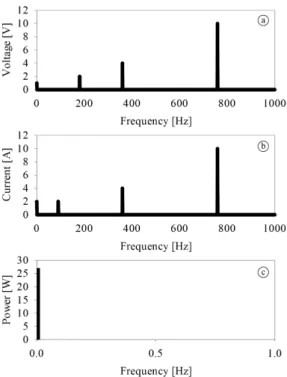
Applying DFT to Equations 17 and 18 in the time domain yields two complex vectors that represent v(wn) and i(wn) in frequency – V(k) and I(k) respectively. The active power is obtained by 1) multiplying the V(k) and I(k) bins at the same position in the frequency vector by the cosine of the phase difference, and 2) adding all such products together. The resulting value represents the active power at zero frequency. Figure 3 shows the absolute values of V(k) and I(k) in frequency, with the active power (P[W]) being presented in zero frequency as 27.00 W.
Both methods can be evaluated to compare the results. DFT using FFT-based computing methodology provides the same results as the mathematical manipulation of the applicable equations. That is explained by the fact that the DFT method allows
the determination of the coeficients of Equation 16,
which are then easily placed into vectors that speed up the obtainment of the required data. Once known, the vectors can be used to solve the active power determination problem through either ordinary hardware or software calculations.
In this simulation the zero-padding process is applied to the same example – Equations 17 and 18 – previously presented. This process does not increase the signal bandwidth, but improves DFT resolution (Lyons, 2010; Spangenberg et al., 2000). In this case the DFT basis functions can better match the original signal and the associated integer frequencies can lie in bins thus minimizing spectrum leakage. The amount
of zero padding inluences computational time as
presented by Spangenberg et al. (2000). In this simulation, a zero padding length of 99,000 was
adopted. This amount proved eficient in resolution
and computational time (Lyons, 2010) by requiring only 18 ms to be processed using a notebook with an Intel Core i5-4210U CPU at 1.7 GHz, cache L1 data with 2×32 kB, L1 inst. with 2×32 kB, Level 2 with 2×256 kB, Level 3 with 3 MB and a DDR3 memory of 8 GB. The results for Simulation 2 are presented in Figure 4.
Following application of zero padding, the respective active power obtained through this approach must be multiplied by the sum of the original signal length and the zero padding length divided by the original signal length [length (original signal + zero padding) / length (original signal)], as expected for a DFT process.
Simulation 3
In this particular case noise has been introduced to the signals while maintaining the zero padding with the same length as in Simulation 2. The new signals are represented by:
( ) ( ) ( )
( 3) ( )1 2
1 10 cos 2 4 cos 2 2 cos 2 v
v t f t f t
f t n t
= + π + π +
π + (19)
( )
( ) ( )
1 2
4
2 10 cos 2 4 cos 2
3 2
2 cos 2 i
i t f t f t
f t n t
π π
= + π + + π + +
π +
(20)
where, n tv( ) ( ) , n ti are the noise signal representation
to voltage and current, respectively. The remaining parameters are the same as in Equations 17 and 18. Noise is provided by a random function in Matlab that generates arrays of random numbers uniformly distributed into the signals. The corresponding result is presented in Figure 5.
As the applied noise signal is a random one the resulting active power follows its variation showing an average of 28.75 W, and a relative error of 6.48%. In order to calculate this average the simulation program ran 100 times (10 times for each of the 10 different zero-padding used lengths) leading to the results presented by Table 1 that shows the accuracy of measurements with different quantities of zero padding. The resulting active power changes with noise and a relative error is computed.
Such error levels are acceptable since the applicable industry standards (Associação…, 2013; International…, 2009) – where the Brazilian standard is fully based on the international one – requires an accuracy of ± 20% if the power is displayed directly on the panel of the electrosurgical unit. According to the same standards, whenever the ESU manufacturer is able to measure power with an error lower than 20%, the Figure 2. Original waveforms from v and i, Equations 17 and 18.
Figure 3. (a) and (b) represent only the magnitudes V(k) and I(k), respectively; (c) The active power in watts is calculated by the sum of the multiplication of the magnitudes of V(k) and I(k) and half of the cosine of the phase difference between V(k) and I(k), for each
actual power value can be displayed accompanied by the inscription “W” that stands for watts. The signals that provided an active power of 28.79 W in Table 1 were also used to simulate coagulation with a duty cycle of 25%. This resulted in an active power of 7.00 W, what represents a relative error of 3.70% in comparison with the value provided by the analytical calculations – 6.75 W. Figure 6 presents the results of such simulation.
Simulation 4
Further studying this approach, the same random noise signal was introduced to both voltage Equation 19 and current Equation 20. This represents the
worst possible situation, as noise will be ampliied.
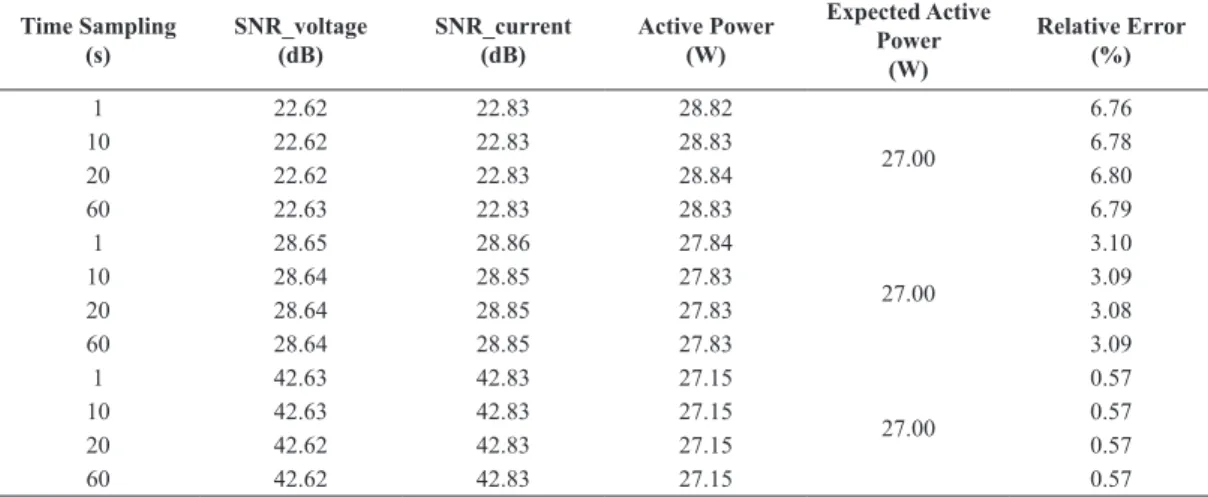
A threshold has not been set to reject power contribution due to the noise, but the simulation was performed considering different noise amplitudes and a total time sampling of 1, 10, 20 and 60 seconds. The average
signal-to-noise ratio (SNR), average active power and relative error, are presented in Table 2. For the worst relative error presented (6.80%) the average active power was 28.84 W, SNR (voltage) was 22.62 dB, and SNR (current) was 22.83 dB.
Practical results
Experimental results during an ablation experience are provided. This experiment was performed by cutting chayote (Sechium edule, SW) (Grande, 2014; Schneider and Abatti, 2008) and swine lesh (Sus domesticus) with energy application through an electrosurgical device built at Federal University of Technology – Paraná (UTFPR) with non-switched output power stage (Bernardi, 2007; Schneider, 2004; Schneider and Abatti, 2005, 2008). The device was able to deliver a quasi-sinusoidal power signal to the tissue. This type of output was selected because
it makes possible to separate inluences such as
Figure 4. (a) and (b) represent only the magnitudes V(k) and I(k), respectively, after applying zero padding; (c) The active power in watts is calculated by the sum of the multiplication of the magnitudes of V(k) and I(k) and half of the cosine of the phase difference between V(k) and
spectral leakage caused by the sparking process. At the same time, it facilitates the calculation of the expected values. In order to acquire the voltage and current signals, energy was applied on a slice of chayote. The adopted frequencies were between 350 and 450 kHz and power between a few watts to a hundred watts (these variables were adjustable in the electrosurgical device). The voltage was sampled on the chayote and the current was sampled through a 7-ohm resistor in series with the chayote. Data was captured by an Agilent Technologies 4-channel oscilloscope model MSO6034A, 300MHz with 2 GSPS and ADC converter (AD converter with 12-bit resolution), with an Agilent 10073c probe (500MHz) for measuring current and a TPI P250 probe 100:1 (250MHz) for measuring voltage. The experiment setup was the same used by Schneider and Abatti (2008). Table 3 shows a set of experiments that were carried out where
chayote (experiments from 22 to 55) and swine lesh
(experiments from 56 to 69) received power through the electrosurgical equipment for ablation. During the ablation procedures, waveforms of the applied voltage and current, ambient temperature as well as tissue mass were recorded (Grande, 2014). This data generated
a ile including 1,000 samples of time with periods
of 10 nanoseconds, voltage and current amplitudes for each of the numbered 22 to 69 experiments. As the experiments included human intervention and considering that the sparking phenomena may present discontinuities, outliers were observed in experiments 22, 25, 38, 50 and 63. All experiments took place in a temperature-controlled laboratory within 27.1 to 27.3 Celsius degrees. Table 4 presents a summary of all experiments.
As a checkpoint, an acquired sinusoidal signal
methodology presented by this paper. The plot for
this ile is presented in Figure 7.
The equations that it the signals of Figure 7 are presented by Equations 21 and 22 (Grande, 2014):
( ) 300.cos 2. . .( 17. / 45)
v t = πf t+ π (21)
( ) 0.09.cos 2. . .( 107. / 180)
i t = πf t+ π (22)
Based on Equation 16 the relations above can be manipulated to lead to P = ((300 × 0.09)/2).
cos(107.π/180-17.π/45), thus P = 10.49 W. Applying the simulation methodology previously presented with zero padding and the same values led to P = 10.82 W. The relative error between both results is just 3.15%,
a igure that is completely acceptable considering that
the actual signal is a little noisy and also taking into account the previous results of Simulations 3 and 4,
which presented relative errors of 6.48% and 6.80%, respectively.
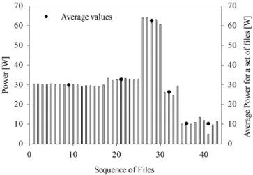
Figure 8 shows the amount of power calculated by the methodology proposed by this paper based on
the sample iles, as well as average values for each
group under consideration. Table 3 summarizes all
sampled iles and delivered power calculated by this
approach in Figure 8.
In order to characterize the signals with or without sparks two measures were made, both using chayote (Sechium edule, SW) as a load for measuring purposes. The experiment setup was the same as previously described. Figure 9 shows the resulting signals in time and frequency domains.
The sparking signals (V1 and I1 in Figure 9) provided an active power of 69.01 W while the non-sparking ones (V2 and I2 in Figure 9) provided 19.94 W. Applying sinusoidal signals allows a better Table 1. Power output with noise changing quantities of zero padding.
Zero-padding
Number of zeros 9000 19000 29000 39000 49000 59000 69000 79000 89000 99000
Active Power [W] (signal with noise)
28.72 28.74 28.77 28.78 28.75 28.78 28.69 28.79 28.75 28.71 28.75 28.72 28.80 28.81 28.63 28.70 28.76 28.70 28.73 28.72 28.77 28.76 28.79 28.73 28.78 28.73 28.74 28.74 28.75 28.71 28.71 28.78 28.75 28.74 28.78 28.77 28.74 28.72 28.73 28.74 28.71 28.74 28.71 28.75 28.77 28.71 28.75 28.72 28.73 28.82 28.78 28.73 28.74 28.71 28.78 28.75 28.77 28.73 28.74 28.80 28.80 28.76 28.76 28.76 28.69 28.70 28.76 28.77 28.68 28.72 28.78 28.77 28.65 28.76 28.74 28.74 28.74 28.74 28.80 28.74 28.78 28.72 28.74 28.71 28.78 28.73 28.72 28.69 28.74 28.71 28.74 28.81 28.69 28.78 28.77 28.77 28.68 28.77 28.79 28.79 Average [W] 28.75 28.75 28.74 28.75 28.75 28.74 28.74 28.74 28.75 28.75
Average Result [W] 28.75
Expected Power [W] 27.00
Relative error 6.48%
Table 2. Active Power and Relative Error considering different amplitude noise and time sampling.
Time Sampling (s)
SNR_voltage (dB)
SNR_current (dB)
Active Power (W)
Expected Active Power
(W)
Relative Error (%)
1 22.62 22.83 28.82
27.00
6.76
10 22.62 22.83 28.83 6.78
20 22.62 22.83 28.84 6.80
60 22.63 22.83 28.83 6.79
1 28.65 28.86 27.84
27.00
3.10
10 28.64 28.85 27.83 3.09
20 28.64 28.85 27.83 3.08
60 28.64 28.85 27.83 3.09
1 42.63 42.83 27.15
27.00
0.57
10 42.63 42.83 27.15 0.57
20 42.62 42.83 27.15 0.57
analysis of the sparking contribution and facilitates understanding of its behavior, what would be very
dificult with switching signals.
Results
Figure 3 presents the result for a known v(t) and i(t), both well behaved signals, after applying the herein presented DFT-methodology based on Equation 15. Such result is exactly the same obtained through the mathematical manipulation of the analytical equation.
Additionally, Figure 4 (Simulation 2) presents the same result as Figure 3 (Simulation 1) after
zero-padding application. Such result is exactly the same, having required only 18 ms of computational time – fast enough to provide feedback to the control system of electrosurgical units for instance.
Figure 5 (Simulation 3) presents the same situation with noise. The average relative error result of 6.48%, presented in Table 1, is in accordance with the applicable industry standard (Associação…, 2013).
not been deined to the noisy signal, active power is
maintained as expected with relative error lower than 7.00%. Table 2 presents these results.
Table 3 presents experimental results produced during the ablation experiment previously explained.
One acquired sampled ile was used to calculate power
using Equation 16 and DFT computing. The relative error was 3.15% actually showing a better result than Simulations 3 and 4.
Based on these results, a set of almost 50 samples of electrosurgical voltage and current signals had its active power determined by the herein presented
method. The results above allow the authors to afirm
that this is a very fast method to determine active Table 3. Sampled iles and delivered power calculated in the ablation experience with the herein proposed method. Negative values were disregarded because of sampling errors by human intervention.
Sequence Sampled File
(txt) Power [W] Sequence
Sampled File
(txt) Power [W]
1 23 30.46 23 47 32.96
2 24 30.54 24 48 32.48
3 26 30.15 25 49 32.90
4 27 30.17 26 51 63.96
5 28 30.61 27 52 64.22
6 29 29.99 28 53 61.47
7 30 30.40 29 54 63.11
8 31 30.18 30 55 60.46
9 32 30.40 31 56 26.17
10 33 30.04 32 57 25.46
11 34 30.04 33 58 24.67
12 35 29.11 34 59 29.42
13 36 29.59 35 60 10.04
14 37 29.56 36 61 10.54
15 39 28.99 37 62 9.95
16 40 28.99 38 64 10.82
17 41 29.91 39 65 13.50
18 42 33.39 40 66 11.95
19 43 32.22 41 67 4.92
20 44 32.58 42 68 9.64
21 45 32.46 43 69 11.33
22 46 33.27
Table 4. Summary of all experiments presented in the Practical Results Section.
Experiment Number Media Quantity Duration (s) Remark
22 to 41 Chayote 14 5
Chayote 6 15
42 to 50 Chayote 9 20
51 to 55 Chayote 5 20 High Power
56 to 59 Swine lesh 4 5 Medium Power (some carbonization
observed)
60 to 69 Swine lesh 10 20
power (real power in watts) for real cases, especially in electrosurgical units.
The methodology to obtain an active power value with less than 10% relative error can be summarized as follows:
1. Acquire signals v(wn) and i(wn) in the time domain;
2. Use DFT to transform v(wn) and i(wn) from the time domain to V(k) and I(k) in the frequency domain and adjust the obtained magnitudes; 3. Calculate the angles (phases) of V(k) and I(k); 4. Calculate active power as (1/2).V(k).I(k).
cos(Δϴ), where Δϴ is the difference between the voltage and current angles, using the simple mathematical multiplication process presented by Equation 16.
Discussion
The herein presented method consists in using DFT as a tool to obtain the moduli and arguments of the frequency components of v(wn) and i(wn) sampled over time on the load (patient) and subsequently applying Equation 16 to determine the active power.
Simulations were performed to evaluate this technique together with sinusoidal electrosurgical output experiments. Simulation 1 represents an ideal situation and the simplest possible application case; it brings the basis to understand how the proposed method works.
Simulation 2 introduced a zero-padding step: once sampled signals are not multiples from 2n, the
zero-padding process was used with a large number of zeros (99,000) for all simulations to allow the DFT basis functions to better match the signal. Its intention
was to show an accurate result and have a generalized process, although mathematical approaches suggest using 2n samples (Lyons, 2010). A zero-padding
comparative method is performed and the resulting active power is presented in Figure 10. The equations were the same of Simulation 4. The simulation program ran 30 times for each group (A, B and C). For the
irst simulation v(wn), i(wn) and noise were the same for each group. For the second simulation v(wn) and i(wn) were maintained and the noise was different for each group, and so on. Group A represents the active power results with original signal length. Group B represents the active power results with original signal length and zero-padding added to perform 2n
samples. Group C represents the active power results with original signal length and 99,000 zero-padding length. Group D represents the expected active power. Figure 10 shows that the performance of the FFT depends only on the input signal’s length and that the length of 2n samples does not make the FFT faster,
as expected, but very close to Group A. The signal length including for Group A was 10,000 samples. The signal length including noise with zero padding to perform 2n samples was 32,768 samples for Group B.
The signal length including noise with 99,000 zero padded was 109,000 samples for Group C. As an
example, the irst active power value calculated for
each of the vectors showed identical results (28.78 W) similarly for the others. However, the execution times were different. For Group A run time was 1.70 ms, for Group B 2.60 ms and for Group C 16.80 ms for the described 28.78 W.
than 99,000 zeros as showed in Figure 10. For this reason, the authors believe that the zero padding
method could be removed without signiicant error
to reduce computational time, what is more important than accuracy in this case, and because the accuracy of the herein proposed method is already better than the industry standard (Associação…, 2013) requires. Additionally, alternatives such as the adjustable window algorithm presented in Hidalgo et al. (2002) or a sliding DFT applied in any time in continuous process (Tang et al., 2006) could be used to reduce computational time. In real applications, reducing computational time is of utmost importance during quasi-real time power regulation.
In the case of ERBE patent (Fritz and Schall, 2014) and Freescale Application Note (Freescale…, 2015), sophisticated, very complex computation is used to obtain the RMS values of voltage and current; a power
factor is then calculated yielding a real component of the current and only after that active power can be calculated. The methodology herein presented requires less computational effort and time than that.
It can be used to certiicate and calibrate electrosurgical
equipment, as well as in generic laboratory checks. This methodology can also be applied to commercial electrosurgical units with or without switching output, providing a relative error lower than 10%.
Additionally, ESUs must comply with tough
technical requirements speciied by industry standards
Manufacturer’s laboratory tests are performed using constant loads and their graphs are presented on the equipment’s operating manuals. In order to certify commercial ESUs, tests are performed using ohmic contact in resistive loads (Associação…, 2013). Although sparking phenomena are not considered in this case they are the ultimate responsible for spectral noise, dc components, dc burns and electrostimulation (Schneider and Abatti, 2008); the herein presented methodology does take that into account as discussed in the ‘Practical results’ section.
The presented methodology can also be used as a reference to compare results as well as an alternative to better control the output power of electrosurgical units.
The most important aspect of the herein proposed method is that it provides a simpler, more effective and faster approach to implement and measure active power when compared to other digital methods. The only way to calculate power through analog circuits is by using new and critical technologies such as logarithm
ampliiers that allow multiplication of two signals –
an essential step in the analogical determination of power. In this case, apparent power [VA] is obtained by multiplying digitized signals v(wn) and i(wn) in time, with the calculation of Equation 2 involving integration of the values of apparent power within a period which corresponds to the calculation of the
area under its curve. This process requires signiicant
computational effort. Furthermore, the DFT application can easily provide the reactive power and the power factor if required.
The herein presented methodology does not include regulation and closed-loop control of the delivered
power. However, it can be used as a step in the control and regulation process of the delivered active power.
In order to avoid errors in the process when using coagulation or another blend mode of the ESU, the circuitry must do the coherent averaging before sampling.
Additionally, this methodology can be used to determine the minimum required power that needs to be delivered to each type of tissue in order to minimize the surgical intervention. It can also be
adopted as part of the ESU certiication procedure
helping manufacturers to improve their equipment. In this particular case an automated system can be implemented to acquire signals in real time and provide feedback to the ESU in order to correct the delivered power aiming at minimizing the harm to the tissue.
The greatest advantage of this methodology is to determine the active power of noisy and phased-out signals, especially those found in commercial, switched electrosurgical devices, without complex DFT or convolution math, without knowing the frequency components generated by the ESU and using less steps that any other existing technique.
Besides that, this method allows the active power
determination during the ESU certiication process
observing the sparking process. The authors believe
that the electrosurgical equipment certiication
process must necessarily consider such process in order to detect problems of asymmetry, DC burns and potential electrical stimulation hazards (Schneider and Abatti, 2008).
Finally, the herein described method is suficiently
general and offers other possibilities of application, being not restricted to the use in electrosurgical units.
References
Abu Khaled M, McCutcheon MJ, Reddy S, Pearman PL, Hunter GR, Weinsier RL. Electrical impedance in assessing human body composition: the BIA method. The American Journal of Clinical Nutrition. 1988; 47(5):789-92. PMid:3364394.
Andria G, Savino M, Trotta A. Windows and interpolation algorithms to improve electrical measurement accuracy. IEEE Transactions on Instrumentation and Measurement. 1989; 38(4):856-63. http://dx.doi.org/10.1109/19.31004.
Associação Brasileira de Normas Técnicas - ABNT. NBR-IEC 60601-2-2: medical electrical equipment part 2-2: particular requirements for the safety of high frequency surgical equipment. Rio de Janeiro: ABNT; 2013. Bernardi R. Desenvolvimento de um equipamento para estudo de eletrocirurgia com controle de potência ativa [dissertation]. Curitiba: Universidade Federal Tecnológica do Paraná; 2007.
Betta G, D’Apuzzo M, Liguori C, Pietrosanto A. An intelligent FFT-analyzer. IEEE Transactions on Instrumentation Figure 10. Zero-padding comparative. Group A, v(wn) and i(wn)
vectors’ original length. Group B, v(wn) and i(wn) and zero-padding to perform 2n samples. Group C, v(wn) and i(wn) and 99,000 zero-padding
and Measurement. 1998; 47(5):1173-9. http://dx.doi. org/10.1109/19.746578.
Chen KF, Cao X, Li YF. Sine wave fitting to short records initialized with the frequency retrieved from Hanning windowed FFT spectrum. Measurement. 2009; 42(1):127-35. http://dx.doi.org/10.1016/j.measurement.2008.04.007.
De Santis V, Beeckman P, Lampasi DA, Feliziani M. Assessment of human body impedance for safety requirements against contact currents for frequencies up to 110 MHz. IEEE Transactions on Biomedical Engineering. 2011; 58(2):390-6. http://dx.doi.org/10.1109/TBME.2010.2066273. PMid:20709636.
Freescale Semiconductor, Inc. FFT-based algorithm for metering applications: AN4255. Eindhoven: NXP Semiconductors; 2015.
Fritz M, Schall H. inventors; ERBE Elektromedizin GmbH, assignee. Electrosurgical gerenator for the treatment of a biological tissue, method for regulating an output voltage of an electrosurgical generator, and corresponding use of the electrosurgical generator. United States patent US 8920412B2. 2014 Dec 30.
Grande KC. Análise da energia utilizada por bisturi elétrico na ablação de tecido orgânico [dissertation]. Curitiba: Universidade Federal Tecnológica do Paraná; 2014.
Harris FJ. On the use of windows for harmonic analysis with the discrete Fourier transform. Proceedings of the IEEE. 1978; 66(1):51-83. http://dx.doi.org/10.1109/PROC.1978.10837.
Hidalgo RM, Fernandez JG, Rivera RR, Larrondo HA. A simple adjustable window algorithm to improve FFT measurements. IEEE Transactions on Instrumentation and Measurement. 2002; 51(1):31-6. http://dx.doi.org/10.1109/19.989893.
Horton JW, VanRavenswaay AC. Electrical impedance of the human body. Journal of the Franklin Institute. 1935; 220(5):557-72. http://dx.doi.org/10.1016/S0016-0032(35)90038-2.
International Electrotechnical Commission. IEC 60990: methods of measurement of touch current and protective conductor current [internet]. 2nd ed. Geneva: IEC; 1999 [cited 2015 Mar 17]. Available from: http://webstore.iec. ch/preview/info_iec60990%7Bed2.0%7Db.pdf
International Electrotechnical Commission. IEC 60601-2-2:2009: medical electrical equipment – Part 2-2: particular requirements for the basic safety and essential performance of high frequency surgical equipment and high frequency surgical accessories [internet]. Geneva: IEC; 2009 [cited 2015 Mar 17]. Available from: http://www.iec.ch/index.htm
Jain VK, Collins WL, Davis DC. High-accuracy analog measurements via interpolated FFT. IEEE Transactions on Instrumentation and Measurement. 1979; 28(2):113-22. http://dx.doi.org/10.1109/TIM.1979.4314779.
Lyons RG. Understanding digital signal processing. 3rd ed. New York: Pearson Education; 2010.
Schneider B Jr, Abatti PJ. Desenvolvimento de um equipamento eletrocirúrgico com saída não chaveada. Revista Brasileira de Engenharia Biomédica. 2005; 21(1):15-24.
Schneider B Jr, Abatti PJ. Electrical characteristics of the sparks produced by electrosurgical devices. IEEE Transactions on Biomedical Engineering. 2008; 55(2 Pt 1):589-93. http:// dx.doi.org/10.1109/TBME.2007.903525. PMid:18269994.
Schneider B Jr. Estudo teórico-prático de parâmetros técnicos e fisiológicos utilizados em eletrocirurgia, visando a otimização do desenvolvimento e performance de um bisturi eletronico [thesis]. Curitiba: Programa de Pós-graduação em Engenharia Elétrica e Informática Industrial, Centro Federal de Educação Tecnológica do Paraná; 2004. Smith KCA, Alley R. Electrical circuits: an introduction. Cambridge: Cambridge University Press. 1992.
Smith SW. The scientist and engineer’s guide to digital signal processing. 2nd ed. San Diego: California Technical Publishing; 1999. v. 1.
Spangenberg SM, Scott I, Mclaughlin S, Povey GJR, Cruickshank DGM, Grant PM. An FFT-based approach for fast acquisition in spread spectrum communication systems. Wireless Personal Communications. 2000; 13(1-2):27-56. http://dx.doi.org/10.1023/A:1008848916834.
Tang X, Zeng X, Tu C. A sliding DFT algorithm for electric power measurement. In: Fang J, Wang Z, editors. Proceedings of SPIE 6357, 6th International Symposium on Instrumentation and Control Technology: Signal Analysis, Measurement Theory, Photo-Electronic Technology, and Artificial Intelligence; 2006 Oct 24; Beijing, China. Beijing: SPIE; 2006. p. 1-5. http://dx.doi.org/10.1117/12.717112.
Authors
André Luiz Regis Monteiro1*, Karin Cristine Grande1, Rubens Alexandre de Faria1, Bertoldo Schneider Junior1
1 Graduate Program in Electrical Engineering and Industrial Informatics, Universidade Tecnológica Federal do Paraná –