Marcelo T. Piovan
[email protected] Centro de Investigaciones en Mecánica Teórica y Aplicada UTN-FRBB, ArgentinaRubens Sampaio
[email protected] Department of Mechanical Engineering PUC-Rio, BrazilJose M. Ramirez
[email protected] Centro de Investigaciones en Mecánica Teórica y Aplicada UTN-FRBB, ArgentinaDynamics of Rotating Non-Linear
Thin-Walled Composite Beams: Analysis
of Modeling Uncertainties
In this article a non-linear model for dynamic analysis of rotating thin-walled composite beams is introduced. The theory is deduced in the context of classic variational principles and the finite element method is employed to discretize and furnish a numerical approximation to the motion equations. The model considers shear flexibility as well as non-linear inertial terms, Coriolis’ effects, among others. The clamping stiffness of the beam to the rotating hub is modeled through a set of spring factors. The model serves as a mean deterministic basis to the studies of stochastic dynamics, which are the objective of the present article. Uncertainties should be considered in order to improve the predictability of a given modeling scheme. In a rotating structural system, uncertainties are present due to a number of facts, namely, loads, material properties, etc. In this study the uncertainties are incorporated in the beam-to-hub connection (i.e. the connection angle and the springs) and the rotating velocity. The probability density functions of the uncertain parameters are derived employing the Maximum Entropy Principle. Different numerical studies are conducted to show the main characteristics of the uncertainty propagation in the dynamics of rotating composite beams.
Keywords: non-linear beams, dynamics, uncertainties, stochastic modeling, rotating composite beams
Introduction
Rotating beams play an important role in the modeling of engineering structures such as turbine blades, airplane propellers and robot manipulators, among others. This subject has been investigated with different levels of intensity and depth, at least, over the last four decades. A historical revision about generally rotating beams can be found in the works of Rao (1987) and Chung and Yoo (2002). In these papers, many epoch-making works are listed as well as recent investigations about rotating beams made of isotropic metallic materials and even composite materials. Simo and Vu-Quoc (1986, 1987) showed that the appropriate consideration of non-linear strain-displacement relationships plays an important role in the correct modeling of the geometric stiffening of flexible beams. It is important to mention that the geometric stiffening has a remarkable effect on the dynamics of rotating and non-rotating beams. Moreover in rotating beams the geometric stiffening is not only due to non-linear strain-displacement relations but also due to centrifugal and Coriolis’ effects (Simo and Vu-Quoc (1987) and Trindade and Sampaio (2002)).
In order to improve the predictability of structural models, different types of mechanical hypotheses have been introduced in the mathematical formulation in the context of deterministic behavior. However, many parameters involved in the formulation, such as modulus of elasticity, density, forces, geometrical measures can be uncertain due to a number of facts such as material production, system construction, system operation and so on. Under these circumstances the quantification of the uncertainty introduced in the mechanics of composite structures plays a crucial role. Many articles addressing uncertainty topics in beam structures were published. Cheng and Xiao (2007) studied the stochastic dynamics of beams subjected to axial loads. Lin (2001) as well as Hosseini and Khadem (2007) studied the reliability of rotating beams with uncertain material properties, uncertain geometric parameters and random rotating speed. Ritto et al. (2008) studied the effect of uncertainty on the boundary conditions
Paper received 10 April 2012. Paper accepted 27 August 2012.
of Timoshenko beams.
There are many papers devoted to dynamic analysis of composite beams, for both rotating and non-rotating conditions, and in some papers, several aspects of uncertainty were tackled. Saravia et al. (2011) analyzed the non-linear dynamics of a rotating thin-walled composite beam. In their paper, the method of multiple scales was employed to obtain the equations with which evaluate the steady responses and their stability. Zibdeh and Abu-Hilal (2003) studied the dynamics of composite beams subjected to random moving loads. Chen and Chen (2001) evaluated the effect of flexure-torsion coupling in the dynamics of rotating composite beams subjected to non-stationary random excitation. Li et al. (2005) analyzed the stochastic response of an axially loaded thin-walled beam with closed cross-section. Murugan et al. (2008) analyzed the aeroelastic response of helicopter blades with random material properties.
of uncertainty in the material properties and the distribution of the reinforcement fibers, the present study is focused on the analysis of uncertainty propagation due to parameters such as stiffness angles, accelerations, velocities, etc. The propagation of the uncertainty in the material properties and laminate features will be part of future research.
Nomenclature
A,L,V = beam domains: area, length and volume ¯
Ai j,Di j¯ = shell elastic properties E∗,G∗ = elasticity moduli of the material J(•) = elastic or mass beam properties
kv,kθ = spring stiffness at hub-to-beam connection Oj = reference center of the frames
Mi j,Ni j = shell forces
u,v = longitudinal and lateral displacement of the bar Vi = generic random variable
F = force vector Pj = material point U = displacement vector
[C] = damping matrix
[K],[KG] = elastic and geometric stiffness matrices
[M],[G] = mass and gyroscopic matrices
Greek Symbols
α = clamping angle
ψ = prescribed rotation of the whole beam ρ = material density
θ = rotation parameter of the cross-section
Mathematical Model
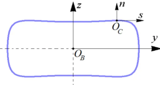
In Fig. 1 one can see a sketch of a rotating beam undergoing arbitrary in-plane rotations, where {OB:xyz}, {OR:xRyRzR} and {OG:xGyGzG}are the local beam frame, rotating frame and inertial fixed frame, respectively. The rotation of the beam is characterized by means of a prescribed rotationψ(t) around thezG-axis. α is the angle that identifies the deviation of the beam axis with respect to the radial direction in the point of the beam-to-hub connection. The cross-section has a doubly symmetric closed contour constructed with layered fiber-reinforced plastic laminates whose mechanics is measured according to the intrinsic frame{OC:xsn}, as shown in Fig. 2.
Figure 1. Reference frames of the rotating beam.
Figure 2. Reference frames of the cross-section.
In order to simplify the model and to concentrate in the stochastic study, the constitutive equations of the composite stacking sequences will be constrained to the cases of especially orthotropic laminates and/or symmetric balanced laminates. With this stacking sequences the possible elastic-constitutive couplings between in-plane (i.e in the plane of rotation) and out-of-plane and/or twisting motions are consistently canceled or, at least, constrained to a negligible amount. The shear strains across the thickness of the wall are neglected as a common assumption in the context of thin-walled modeling. Under these circumstances the stress-strain equations can be reduced to the following form:
Nxx Nxs Mxx Mxs
=
¯
A11 . . .
. A¯66 . .
. . D¯11 .
. . . D¯66
¯ εxx
¯ γxs
¯ κxx
¯ κxs
(1)
In Eq. (1)NxxandNxsare membrane forces whereasMxxandMxs are shell moments defined according to Eq. (2). On the other hand, ¯
εxx,γ¯xs,κ¯xxandκ¯xsare shell strains and shell curvatures.
{Nxx,Nxs}= ˆ
e
{σxx,σxs}dn,
{Mxx,Mxs}=
ˆ
e
n{σxx,σxs}dn,
(2)
The coefficients A¯11, A¯66, D¯11 and D¯66 are modified elastic coefficients of the shell, re-defined according to Piovan and Cortínez (2007). According to the configuration selected, one can prove (Cortínez and Piovan, 2002) that, for closed cross-sections, the expressions of the effective longitudinal (E∗) and transversal (G∗) elasticity moduli can be written in terms of the laminate elastic coefficients as:
E∗=A¯11
e =
12D¯11
e3 , G∗= ¯ A66
e (3)
In Eq. (2) and Eq. (3) eis the thickness of the wall, which is assumed constant and deterministic in this paper.
For a beam rotating around theZG-axis, the position vector of a generic pointP, of the beam domain, with respect to the inertial frame
PG(Px|G,Py|G)and with respect to the rotating frame PR(Px|R,Py|R) may be written as:
PG= [TG]PR,
PR= [TR] (U+XB) +R,
where:
[TR] =
cosα −sinα
sinα cosα
,
[TG] =
cosψ(t) −sinψ(t)
sinψ(t) cosψ(t)
, U= ux uy ,XB=
x y
,R=
R0 0 , (5)
In Eq. (5),uxanduyare the displacements of a generic point of the deformed configuration measured with respect to the local frame
{OD:xyz}, that is:
ux(x,y,t) =u(x,t)−yθ(x,t)
uy(x,y,t) =v(x,t) . (6)
The variablesu,vandθare the extensional displacement, lateral displacement and bending rotation of the cross-section, respectively. As one can easily see, Eq. (6) is describing a typical shear-deformable, or Timoshenko’s formulation.
According to the nomenclature of thin-walled beams, the coordinates of a point in the cross-sectional plane, let’s sayB(y,z), can be defined in the intrinsic frame{OC:xsn}as:
y(s,n) =Y(s)−ndZ(s)
ds ,z(s,n) =Z(s) +n dY(s)
ds , (7)
whereY(s)andZ(s)are the coordinates of the middle line of the shell contour.
Taking into account the definition of the Lagrangian strain tensor and the Eq. (6), one can obtain the relevant components of the strain tensor as:
εxx=u′−yθ′+12 h
(u′−yθ′)2+v′2 i
γxy= (v′−θ)−[θ(u′−yθ′)]
. (8)
For convenience in the algebraic handling, the strain components of Eq. (8) should be transformed and described in the intrinsic frame
{A:xsn}, that is,εxxandγxs, which can be written in the following form:
S= ([DL] +n[BL])SL+
[DNL] +n[BNL] +n2[BNL2]
SNL (9)
with
S={εxx,γxs}T, SL={u′,θ′,v′−θ}T, SNL=
u′2,v′2,θ′2,u′θ′,θ′θ,u′θ T
[DL] =
1 −Y 0
0 0 dZ/ds
,[BL] =
0 dZ/ds 0
0 0 0
,
[DNL] =
1/
2 1/2 1/2Y2 −Y 0 0
0 0 0 0 YdZ/ds −dZ/ds
,
[BNL] =
0 0 −YdZ/ds dZ/ds 0 0
0 0 0 0 (dZ/ds)2 0
,
[BNL2] =
0 0 1/2(dZ/ds)2 0 0 0
0 0 0 0 0 0
.
(10)
The velocity vector of a generic point can be obtained from (4) in the following form:
dPG dt =
˙
PG=ψ˙[TG2]PR+ [TG] [TR]U˙ (11)
where:
[TG2] =
−sinψ(t) −cosψ(t)
cosψ(t) sinψ(t)
(12)
In Eqs. (8), (11) and in the following paragraphs, dots and apostrophes identify derivatives with respect to time and space (i.e. x), respectively.
Now the total potential energy (composed of strain energy and energy stored by root stiffness) and the kinetic energy of a composite rotating beam can be described as:
UD= 1
2 ˆ
V
ST[EM]SdV+kv
2v 2
(0,t) +kθ
2θ 2
(0,t),
UK= 1
2 ˆ
V
ρP˙G·P˙GdV,
(13)
where[EM] =diag[E∗,G∗], whereasE∗,G∗andρare the Young’s modulus, shear modulus and material density, respectively. E∗and G∗are given in Eq. (3). In order to account for the effective shear stress distribution according to a first-order-shear beam formulation, the shear modulus can be affected by the factorκ, which is a class of Timoshenko’s shear coefficient that can be consistently calculated, for composite beams, following the methodology given by Piovan and Cortínez (2005) or Cortínez and Piovan (2002).
Now, substituting Eqs. (8) and (11) into Eq. (13), one obtains:
UD= 1
2 ˆ
L
h
J11Eu′2+J22Eθ′2+J11G v′−θ 2i dx+ 1 2 ˆ L J11E
u′3+u′v′2−3J22Eu′θ′2 dx− 1 2 ˆ L h
2J11G v′−θ
u′θ+J22Gθ2θ′2 i dx+ 1 2 ˆ L " J11E
4
u′2+v′2 2
+J
E 33θ′4
4 # dx+ 1 2 ˆ L " J22Eθ′2
2
3u′2+v′2
+J11Gu′2θ′2 #
dx+
1 2 h
kvv2(0,t) +kθθ2(0,t)
i ,
UK= 1
2 ˆ
L
J11ρ hu˙2+v˙2+2ψ˙(v˙(u+x+R0Cα))
i dx+
1 2 ˆ
L
J11ρ hψ˙2u2+v2−2ψ˙u˙(v+R0Sα)
i dx+
1 2 ˆ
L
J11ρ h
˙ ψ2
2ux+x2+R20 i
dx+
1 2 ˆ
L
J11ρ h2ψ˙2((u+x)R0Cα−vR0Sα)
i dx+
1 2 ˆ
L
J22ρ hθ˙2+2θ˙ψ˙+1+θ2ψ˙2idx,
(15)
where for simplification purposes,Cα=cosαandSα=sinαand:
n
JE,JG,Jρo=
ˆ
A
{E∗,G∗,ρ}gTgdsdn,g=n1,y,y2oT. (16)
In order to calculate the elastic and inertial properties of the cross-section, one should employ in Eq. (16) the definitions given in Eq. (7). For more details, the interested reader should see Cortínez and Piovan (2002).
The non-linear equations of motion can be derived by means of the Hamilton’s principle, i.e.:
δ t2
ˆ
t1
(UK−UDR)dt=0, (17)
whereUDRis the reduced strain energy derived from Eq. (14) in which the double underlined terms are assumed negligible as in other papers devoted to study rotating beam made of isotropic materials (Trindade and Sampaio, 2002). This viewpoint is consistently discussed in a study of the geometric stiffening effect in flexible beams carried out by Mayo et al. (2004). If all underlined terms of Eq. (14) are removed, a linear formulation is obtained.
Finite Element Discretization
Computational models can be constructed through the discretization of the Eq. (17) by an appropriate scheme. The discretization is carried out using a 2-node finite element with three kinematic variables at each node. Lagrange linear shape functions (Nu), cubic shape functions (Nv) and quadratic shape functions (Nθ) are employed for axial displacements, lateral displacements and bending rotations, respectively, i.e:
u=Nuqe, v=Nvqe, θ=Nθqe,
(18)
where:
qe={u1,v1,θ1,u2,v2,θ2}T,
Nu={1−ξ, 0, 0,ξ, 0, 0}, Nv=
0,1+β(1−ξ1+)−β3ξ2+2ξ3,[2+β−(4+β)ξ+2ξ
2]ξL
e
2(1+β) ,
0,βξ+31+ξ2β−2ξ3,[−β+(β−2)ξ+2ξ
2]ξL
e 2(1+β)
,
Nθ=
0,6Lξe(1+(ξ−β1)),[1+β−(4+β)ξ+3ξ
2]
1+β ,
0,−6Lξe(1+(ξ−β1)),(−2+1+β+3βξ)ξo,
(19)
Leis the length of the generic element,ξandβare defined as:
ξ= x
Le, β=
12J22E L2
eJ11G
. (20)
The shape functions of Nv and Nθ (that correspond to a
Timoshenko’s beam theory or to a typical first-order shear deformable beam theory) are thoroughly introduced in the works of Przemieniecki (1968) and Bathe (1982). On the one hand, the interpolating functions give a consistent integration of the equations of a shear-deformable isotropic beam, as one can see in the aforementioned references. On the other hand, it was shown that they can be useful also for shear-deformable composite beams (Piovan and Cortínez, 2007). In both cases, avoiding the shear-locking effect. Moreover,Nv andNθcan
also be employed to approximate the solution of a Bernoulli-Euler beam equation, because the interpolating functions may be reduced to cubic and quadratic Hermite’s polynomials, if the condition of infinite shear stiffness (orβ→0) is invoked (Przemieniecki, 1968).
Now, substituting Eq. (18) in Eqs. (14) and (15), after performing the conventional steps of variational calculus in Eq. (17) one gets the equation for a single finite element in the following form:
[Me]q¨e−ψ˙[Ge]q˙e+ ([Ke] + [Kg(qe)])qe− ˙
ψ2[Me] +ψ¨[Ge]
qe=ψ˙2f A−ψf¨ T,
(21)
where
[Me] =
ˆ 1
0 h
J11ρ
NTuNu+NTvNv
+Jρ22NθTNθ
i
Ledξ, (22)
[Ge] =2 ˆ 1
0 h
J11ρ NTuNv−NTvNu i
Ledξ, (23)
[Ke] =
ˆ 1
0 h
J11EN′ T
uN′u+J22EN′ T θN′θ
i 1
Ledξ+ ˆ 1
0 h
J11GN′Tv−LeNTθ N′v−LeNθ
i 1 Ledξ
[Kg] =
ˆ 1
0 JE
11 2L2 e h
3N′TuN′uqeN′u+N′TuN′vqeN′v i
dξ+
ˆ 1
0 JE11 2L2 e h
N′TvN′uqeN′v+N′TvN′vqeN′u i
dξ+
ˆ 1
0 3J22E
2L2 e h
N′TuN′θqeN′θ+N′ T
θN′uqeN′θ
i dξ+
ˆ 1
0 3J22E
2L2 e h
N′θTN′θqeN′u i
dξ−
ˆ 1
0 J11G 2Le h
N′TuNθqe N′v−LeNθ i
dξ−
ˆ 1
0 J11G 2Le h
N′Tu N′v−LeNθ
qeNθ
i dξ−
ˆ 1
0 J11G 2Le h
NθTN′uqe N′v−LeNθ
i dξ−
ˆ 1
0 J11G 2Le h
+NTθ N′v−LeNθ
qeN′u
i dξ−
ˆ 1
0 J11G 2Le
h
N′Tv−LeNθTNθqeN′u i
dξ−
ˆ 1 0 JG 11 2Le h
N′Tv−LeNTθ
N′uqeNθ
i dξ,
(25)
fA= ˆ 1
0 h
J11ρNTu(Leξ+R0Cα)−Jρ11N T vR0Sα
i
Ledξ, (26)
fT= ˆ 1
0 h
Jρ11NTv(Leξ+R0Cα)
i Ledξ+
ˆ 1
0 h
Jρ11NTuR0Sα+J22ρNTθ
i Ledξ.
(27)
After the assembling process one gets the following expression:
[M]Q¨ + [C]Q˙ + ([K] + [KG(Q)] + [KD])Q=F, (28)
where[M]is the global mass matrix, [C]is the global gyroscopic matrix,[K]is the global elastic stiffness matrix, [KG]is the global geometric stiffness matrix,[KD]corresponds to the stiffness induced by the rotation of the beam andFis the global vector of dynamical forces. One may notice that[KD]is not symmetric due to the presence of the term proportional to the angular accelerationψ¨.
The matrix [C] can be modified in order to account for "a posteriori" structural damping, i.e.:
[C] = [G] + [CRD]. (29)
In the previous equation, [G] is the global gyroscopic matrix, whereas[CRD]is the system proportional damping matrix, which is calculated as:
[CRD] =η1[M] +η2[K]. (30)
The coefficientsη1andη2can be computed from modal damping coefficients (namely,ξ1 andξ2, from experiments) for the first and second frequencies according to the common methodology presented in the bibliography, related to finite element procedures (Bathe, 1982)
and vibration analysis (Meirovitch, 1997). Remember that[M] is the global mass matrix and[K]is the global elastic stiffness matrix. The Matlab Odesuite is employed to numerically simulate the finite element model, for this reason Eq. (28) is represented in the following form:
[A]dW
dt + [B]W=D, (31)
where:
[A] =
[C] [M] [M] [0]
,
[B] =
[K] + [KG(Q)] + [KD] [0] [0] −[M]
, W= Q ˙ Q , D=
F 0 . (32)
Equation (31) is subjected to the initial conditionW=W0.
Probabilistic Model
In this article the Maximum Entropy Principle (MEP) is employed in order to construct the probabilistic model for the uncertain parameters. Three parameters related to the beam-to-hub connection will be chosen as uncertain: the springs stiffness (kv and kθ) at
the hub, the connection angleα. Also three parameters connected with the rotational angle ψ will be considered uncertain. These parameters characterize the angular acceleration of the angular velocity. Depending on the type of rotating law associated with angle
ψone or two kinematic parameters are introduced. The stiffnesses will be considered unbounded positive random variables and the two angles bounded random variables. The random variablesV1,V2, and V3, related to constructive aspects, as well as random variablesV4,
V5andV6, related to the kinematics, are introduced to construct the
probability models. The random variablesV1andV2identify the hub stiffnessesskvandkθ,V3 is associated with the connection angleα, whereas random variableV4identifies the parameter of a rotation rule with constant acceleration/deceleration segments, and finally random variablesV5 andV6 identify time and opening angle parameters of a rotation law with smooth variation. Depending on the type of rotational law involved a probabilistic model with four (V1,V2,V3and
V4) or five (V1,V2,V3,V5andV6) random variables will be employed.
The available information to prepare the probabilistic model is that the mean value of each random variable is known, i.e. E(Vi) =V
i, and that each random parameter is considered positive. Then, using the MEP and the information that the random variablesVi,i=1, ..., 6 are supposed to be positive, the MEP gives the result that they must be independent. Consequently, the probability density function for random variablesV1 andV2, using the MEP, leads to (Ritto et al., 2008; Soize, 2001):
pVi(vi) = 1]0,∞](vi)
δV−2
i δVi−2
ViΓδ−2 Vi
vi Vi
δ−2Vi−1
×
×exp − vi
δ2V
iVi !
,Vi=
kv,i=1 kθ,i=2
whereδViandVi,i=1, 2 are the dispersion parameter and the mean value of the random variableVi. 1]0,∞](vi)is the support function of the random variable andΓ(ζ) =´∞
0 t
ζ−1e−tdtis the gamma function
defined forζ>0. The dispersion parametersδV1andδV2are confined
in the range 0,√1/3
. This is due toV1 andV2 must be random variables of second order. SinceV3andV4andV5andV6are bounded the MEP says they are distributed uniformly. Thus, the distribution of random variablesVi,i=3, ..., 6 can be written in the following generic form:
pVi(vi) =1[LVi,UVi] (vi) 1 2√3ViδVi
,i=3, ..., 6 (34)
where1[L
Vi,UVi] (vi)is the generic support function, whereas
LV
iand
UV
i are the lower and upper limits of the random variableVi. Once againδViandViare the dispersion parameter and the mean value of the random variableVi,i=3, ..., 6.
The Matlab function gamrnd1/δ2 Vi,δ
2 ViVi
can be used to generate the realizations of the random variables V1, and V2, according to Eq. (33), whereas the function unifrndVi 1−δVi
√
3
,Vi 1+δVi
√
3
can be used to generate realizations for the random variablesV3,V4,V5andV6.
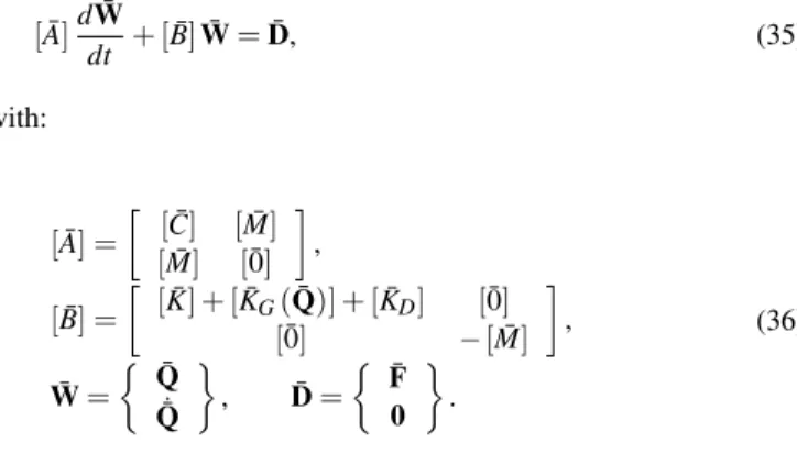
Then, employing Eq. (33) and Eq. (34) into the finite element model given in Eq. (28) and then in Eqs. (31)-(32), the stochastic finite element model is finally written as:
[A¯]d
¯ W dt + [
¯
B]W¯ =D¯, (35)
with:
[A¯] =
[C¯] [M¯]
[M¯] [0¯]
,
[B¯] =
[K¯] + [K¯
G(Q¯)] + [KD¯ ] [0¯]
[0¯] −[M¯]
,
¯ W=
¯
Q ˙¯ Q
, D¯ =
¯
F 0
.
(36)
where, the bar over the vectors and matrices identifies the random coefficient. Thus, the stiffness matrix [K¯] is random due to the presence of random variablesV1 and V2, whereas matrix [KD¯ ] is random due to random variablesV3andV4(orV5andV6depending on the case). The matrix[C¯]is random due toV
4(orV5andV6) and due to the random characteristics of[K¯]. The geometric stiffness matrix
[K¯
G(Q¯)]is random due to the random nature of the displacementsQ¯. The force vectorF¯ is random due to random variablesV3andV4(or V5andV6).
The Monte Carlo method is used to simulate the stochastic dynamics, which implies the integration of a deterministic system for each realization of random variablesVi,i=1, ..., 6. Recall that the probabilistic model can be of four or five random variables depending on the rotation rule selected. In order to control the quality of the simulation process within a prescribed level of approximation, the mean-square convergence of the stochastic response Q¯ has to be evaluated. The convergence is calculated appealing to the following function:
conv(NMS) = v u u t
1 NMS
NMS
∑
j=1ˆ t1
t0
Q¯j(t)
2
dt (37)
whereNMSis the number of Monte Carlo samplings.
Numerical Studies
For the numerical studies a composite box-beam with rectangular cross-section is employed. The measures of the cross-section are such that Ly=3Lz=3cm and the wall-thickness isen =2mm. The beam is constructed with graphite fiber reinforced epoxy resin AS4/3501, whose material properties are: E1 =144 GPa, E2 = 9.65 GPa, G12 =4.14 GPa, G13 =4.14 GPa, G23 =3.45 GPa,
ν12=0.3;ν13=0.3;ν23=0.5;ρ=1389kg/m3. The considered laminate schemes are {0/0/0/0}, {0/90/90/0} and {45/-45/-45/45}. For qualitative comparison purposes the configuration of the rotating beam and the hub radius is restricted toL+R0=1.2mwithR0/L∈
[0.2, 1.0].
In the following examples, models of 20 finite elements are employed to perform the deterministic calculations of each realization in the Monte Carlo Method. It was shown (Piovan, 2003) that with the interpolation functions of Eq. (19) in the finite elements, it is needed a mesh of no more than 20 elements in order to achieve a precision of 99% in the first six natural frequencies. Another important topic is to ensure the convergence of the Monte Carlo simulation in the sense of the norm given by Eq. (37). A convergence analysis was performed for a given set of dispersion parameters, and it was verified that the approximation converges forNMS=400 for a prescribed precision of 99%, although in some cases even withNMS=200 it is possible to reach the prescribed precision. In Fig. 3 it is possible to see an example of the convergence in the sense of the mean-square.
0 50 100 150 200 250 300 350 400
5 5.2 5.4 5.6 5.8 6 6.2 6.4x 10
−7
NMS
conv(N
MS
)
Figure 3. Convergence in the mean-square sense .
The first case corresponds to a beam that rotates following the rule:
˙ ψ=
At, ∀t∈[0, 2)
A(4−t), ∀t∈[2, 4]
0, ∀t>4
(38)
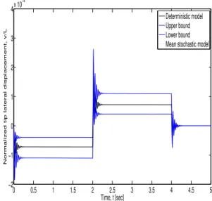
whereA=V4is a uniform random variable. In Fig. 4 one can see the tip lateral displacement of a rotating beam constructed with the stacking sequence {0/0/0/0}, with R0/L =0.2 and the following mean values in the random parameters: V1=V2=102max([Kii]), V3=0.1radandA=V4=5.0rad/s2. The stochastic simulation was performed with 400 samplings and a coefficient of variation
δVi=σVi/Vi=0.05,i=1, ..., 4. Clearly,σViis the standard deviation ofVi, i=1, ..., 4. In Fig. 5 one can see the same response of the previous figure but for coefficient of variationδVi =0.1. In both figures, the upper and lower bounds of the 98% confidence interval are shown.
0 0.5 1 1.5 2 2.5 3 3.5 4 4.5 5
−1.5 −1 −0.5 0 0.5 1 1.5 2x 10
−4
Time, t [sec]
Normalized tip lateral displacement, v/L
Deterministic model Upper bound Lower bound Mean stochastic model
Figure 4. Tip displacement history for a composite beam that rotates
according to Eq. (38), forδVi=0.05in all variables.
Other studies were carried out by analyzing the propagation of uncertainty due to the aforementioned random variables, but one by one separately. For example in Fig. 6(a) one can see the influence of only the random variableV3 (i.e. clamping angleα), whereas in Fig. 6(b) one can see the influence of solely the random variable V4 (i.e. the speed of the positioning angle). In both cases the same variation coefficientδ=0.05 was employed. It is noticeable that the propagation of the uncertainty due to the positioning angle parameter is the most relevant and the uncertainty due to the stiffness parameters at the beam-to-hub connection is not quite relevant.
The previous analysis was done for a rotating beam with a step-wise acceleration, which depending on the case could have a high oscillatory response, with high stress gradients that could eventually lead to failure. Other type of rotation rules can avoid high oscillatory response if the acceleration, velocity and position angle can vary smoothly like in the following rule:
0 0.5 1 1.5 2 2.5 3 3.5 4 4.5 5
−2 −1 0 1 2 3 4x 10
−4
Time, t [sec]
Normalized tip lateral displacement, v/L
Deterministic model Upper bound Lower bound Mean stochastic model
Figure 5. Tip displacement history for a composite beam that rotates
according to Eq. (38), forδVi=0.1in all variables.
˙
ψ(t) =ψ0π
2T0
sin
πt T0
−1
2sin
2πt T0
(39)
In Eq. (39), two possible sources of uncertainties can be taken into account. The first can be identified as the spread angleψ0, and the second can be recognized as the positioning timeT0. These sources of uncertainty are here considered with random variablesV5andV6 having uniform distribution. Also, random variablesV5 andV6are independent and not correlated. Then, the probabilistic model for this case has in common with the previous study the random variablesV1, V2andV3.
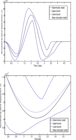
In Fig. 7 one can see the stochastic transient response of composite beam with the same features of the previous study for variation coefficientδ=0.02 in all random variables, i.e. V1,V2, V3,V5andV6. The mean values of the random variablesV5andV6are V5=2.0secandV6=2.0rad. In Fig. 8 the stochastic response for a variation coefficientδ=0.05 is shown. In both figures the upper and lower bounds of the 95% confidence interval are included.
As well as in the previous example with the step-wise acceleration rule, in the case of Eq. (39) the influence of different random variables in the propagation of the uncertain response was evaluated. Thus, in Fig. 9(a) one can see the influence of only random variableV3 for a variation coefficientδV3=0.05; on the other hand, in Fig. 9(b) one
can see the uncertainty propagation related to random variablesV5and V6, also with a variation coefficientδV5=δV6=0.05. In both cases
the 95% confidence interval was included. The difference between the cases are remarkable. A comparison between Fig. 9 and Fig. 8(a) implies that the uncertainty in the response can propagate more due to kinematic parameters (actually,V5 andV6) than due to geometric parameters (actually,V3orV1andV2).
Conclusions
0 0.5 1 1.5 2 2.5 3 3.5 4 4.5 5 -1.5
-1 -0.5 0 0.5 1 1.5 2
Time, s [sec]
tip
lateral
displacement,
v/L
[m] Deterministic model
Upper bound Lower bound Mean stochastic model x 10-4
N
ormalized
(a)
0 0.5 1 1.5 2 2.5 3 3.5 4 4.5 5 −1.5
−1 −0.5 0 0.5 1 1.5 2 2.5x 10
−4
Time, t [sec]
Normalized tip lateral displacement, v/L
Deterministic model Upper bound Lower bound Mean stochastic model
(b)
Figure 6. Tip displacement history for a composite beam that rotates
following Eq. (38), forδVi=0.05(a) only in random variableV3, (b) only in
random variableV4.
behavior of a composite structure. The effect of the uncertain parameters such as beam-to-hub connection stiffness, angle of clamping and positioning angle (speed and/or acceleration) has been studied. From the different studies carried out some points should be remarked:
• The propagation of uncertainty in the tip displacement of the transient response, due to stiffness parameterskvandkθ, is very
small.
• The propagation of uncertainty due to the random variable associated with the angle of the beam-to-hub connection is more important than the influence of the uncertainty in the stiffness parameters.
• The propagation of uncertainties due to the random variables associated with the positioning angle (as well as angular velocity and/or acceleration) is quite remarkable.
• The propagation of uncertainty in the transient response due to
0 0.5 1 1.5 2 2.5 3 3.5 4 4.5 5 −6
−4 −2 0 2 4 6 8x 10
−5
Time, t [sec]
Normalized tip lateral displacement, v/L
Deterministic model Upper bound Lower bound Mean stochastic model
Figure 7. Tip displacement history for a composite beam that rotates
following Eq. (39), forδVi=0.02in all variables.
the clamping parameters altogether is small in comparison to the uncertainty propagation associated with the positioning angle (velocity, acceleration) parameters.
Other features of the model itself can be subjected to uncertainty, as for example the orientation of the reinforcing fibers or the uncertainty of material constituents (elasticity modulus, material density, etc.). On the one hand, many of these parameters can be treated as random variables, although there is an uncertainty related to the model and in this context a more sophisticated analysis tool should be employed, for example the non-parametric probabilistic approach. On the other hand, the material properties along the beam can vary due to uncertainties in the composite fabrics and the construction process; that leads to a stochastic field, then Markov-chain and Monte Carlo method should be taken into consideration to face at this particular problem. However, these topics are the matter of ongoing works.
Acknowledgements
The authors gratefully acknowledge the support of the following Argentinean and Brazilian institutions: Consejo Nacional de Investigaciones Científicas y Técnicas (CONICET), Secretaría de Ciencia y Tecnología, Universidad Tecnológica Nacional,Conselho Nacional de Desenvolvimento Científico e Tecnológico(CNPQ) and Fundação de Amparo à Pesquisa do Estado do Rio de Janeiro (FAPERJ).
References
Bathe, K., 1982, “Finite element procedures in engineering analysis”. Prentice-Hall, Englewood Cliffs, USA.
Chen, C., Chen, L., 2001, “Random response of a rotating composite blade with flexure-torsion coupling effect by the finite element method”, Composite Structures, Vol. 54, pp. 407-415.
0 0.5 1 1.5 2 2.5 3 3.5 4 4.5 5 −6
−4 −2 0 2 4 6 8 10 12x 10
−5
Time, s (sec)
Normalized tip lateral displacement, v/L
Deterministic model Upper bound Lower bound Mean stochastic model
(a)
2.8 2.9 3 3.1 3.2 3.3 3.4 3.5 −4.5
−4 −3.5 −3 −2.5 −2 −1.5
x 10−5
Time [sec]
Normalized tip lateral displacement, v/L
Deterministic model Upper bound Lower bound Mean stochastic model
(b) Figure 8. (a) Tip displacement history for a composite beam that rotates following Eq. (39), forδVi=0.05in all variables, (b) a detail.
Cortínez, V., Piovan, M., 2002, “Vibration and buckling of composite thin walled beams with shear deformability”,Journal of Sound and Vibration, Vol. 258, No. 4, pp. 701-723.
Hosseini, S., Khadem, S., 2007, “Vibration and reliability of a rotating beam with random properties under random excitation”,International Journal of Mechanical Sciences, Vol. 49, No. 12, pp. 1377-1388.
Li, J., Wu, G., Shen, R., Hua, H., 2005, “Stochastic bending-torsion coupled response of axially loaded slender composite-thin-walled beams with closed cross-sections”,International Journal of Mechanical Sciences, Vol. 47, No. 1, pp. 134-155.
Lin, S., 2001, “The probabilistic approach for rotating timoshenko beams”,International Journal of Solids and Structures, Vol. 38, No. 40-41, pp. 7197-7213.
Mayo, J., Garcia-Vallejo, D., Domínguez, J., 2004, “Study of the geometric stiffening effect: Comparison of different formulations”,Multibody System Dynamics, Vol. 11, No. 4, pp. 321-341.
Meirovitch, L., 1997, “Principles and Techniques of Vibrations”, Prentice-Hall Inc., USA.
Murugan, S., Ganguli, D., Harursampath, D., 2008, “Aeroelastic response of helicopter rotor with random material properties”,Journal of Aircraft, Vol. 45, No. 1, pp. 306-322.
Piovan, M., 2003, “Estudio teórico y computacional sobre la mecánica de vigas curvas de materiales compuestos, con sección de paredes delgadas,
0 0.5 1 1.5 2 2.5 3 3.5 4 4.5 5
-4 -2 0 2 4 6 8
Time, t [sec] x 10-5
tip
lateral
displacement,
v/L
N
ormalized
Upper bound Lower bound Mean stochastic model Deterministic model
(a)
0 0.5 1 1.5 2 2.5 3 3.5 4 4.5 5 -5
0 5 10
Time, t [sec]
tip
lateral
displacement,
v/L
N
ormalized
Deterministic model Upper bound Lower bound Mean stochastic model x 10-5
(b)
Figure 9. Tip displacement history of a composite beam that rotates
following Eq. (39) forδVi=0.05(a) only in random variableV3, (b) in random
variablesV5andV6.
considerando efectos no convencionales”, Phd. thesis, Departamento de Ingeniería Universidad Nacional del Sur, Argentina.
Piovan, M., Cortínez, V., 2005, “The transverse shear deformability in dynamics of thin walled composite beams: consistency of different approaches”,Journal of Sound and Vibration, Vol. 285, No. 3, pp. 721-733.
Piovan, M., Cortínez, V., 2007, “Mechanics of shear deformable thin-walled beams made of composite materials”,Thin-Walled Structures, Vol. 45, No. 1, pp. 37-72.
Przemieniecki, J., 1968, “Theory of matrix structural analysis”, McGraw-Hill Company, New York, USA.
Rao, J., 1987, “Turbomachine blade vibration”,The shock and vibration digest, Vol. 19, No. 3, pp. 3-10.
Ritto, T., Sampaio, R., Cataldo, E., 2008, “Timoshenko beam with uncertainty on the boundary conditions”,Journal of the Brazilian Society of Mechanical Sciencesand Engineering, Vol. 30, No. 4, pp. 295-303.
Saravia, C., Machado, S., Cortínez, V., 2011, “Free vibration and dynamic stability of rotating thin-walled composite beams”, European Journal of Mechanics, A/Solids, Vol. 30, No. 3, pp. 432-441.
Simo, J., Vu-Quoc, L., 1986, “A three dimensional finite-strain rod model. part ii: computational aspects”,Computer Methods in Applied Mechanics and Engineering, Vol. 58, No. 1, pp. 79-116.
dynamic analysis of flexible structures”,Journal of Sound and Vibration, Vol. 119, No. 3, pp. 487-508.
Soize, C., 2001, “Maximum entropy approach for modeling random uncertainties in transient elastodynamics”,Journal of Acoustical Society of America, Vol. 109, No. 5, pp. 1979-1996.
Trindade, M., Sampaio, R., 2002, “Dynamics of beams undergoing large rotations accounting for arbitrary axial deformation”,Journal of Guidance, Control and Dynamics, Vol. 25, No. 4, pp. 634-643.