Ricardo de Medeiros
[email protected] University of São Paulo Engineering School of São Carlos Department of Aeronautical Engineering 13563-120 São Carlos, SP, BrazilMariano E. Moreno
[email protected] Federal University of São Carlos Center of Exact Sciences and Technology 13565-905 São Carlos, SP, BrazilFlávio D. Marques
[email protected] University of São Paulo Engineering School of São Carlos Department of Aeronautical Engineering 13563-120 São Carlos, SP, BrazilVolnei Tita
[email protected] University of São Paulo Engineering School of São Carlos Department of Aeronautical Engineering 13563-120 São Carlos, SP, BrazilEffective Properties Evaluation for
Smart Composite Materials
The purpose of this article is to present a method which consists in the development of unit cell numerical models for smart composite materials with piezoelectric fibers made of PZT embedded in a non-piezoelectric matrix (epoxy resin). This method evaluates a globally homogeneous medium equivalent to the original composite, using a representative volume element (RVE). The suitable boundary conditions allow the simulation of all modes of the overall deformation arising from any arbitrary combination of mechanical and electrical loading. In the first instance, the unit cell is applied to predict the effective material coefficients of the transversely isotropic piezoelectric composite with circular cross section fibers. The numerical results are compared to other methods reported in the literature and also to results previously published, in order to evaluate the method proposal. In the second step, the method is applied to calculate the equivalent properties for smart composite materials with square cross section fibers. Results of comparison between different combinations of circular and square fiber geometries, observing the influence of the boundary conditions and arrangements are presented.
Keywords: smart composite materials, piezoelectric fiber composite, active fiber
composite, finite element analyses, effective properties
Introduction
Smart composites present great potential for applications in aerospace industry. Among the alternatives to achieve such concept, there are active fiber composite (AFC) actuators developed by MIT (Bent, 1993), and macro-fiber composite (MFCTM) actuators constructed at NASA Langley Research Center (Wilkie et al., 2000). These materials have been largely investigated during the last years. Piezoelectric materials (also denoted as PZT) have the property of converting electrical energy into mechanical energy, and vice versa (Berger et al., 2005). This capability allows applications as sensors or actuators in several industrial fields, for example: noise and vibration control, acoustic speakers, precision position control and structural health monitoring (SHM). Several approaches (experimental, analytical, numerical or hybrid) have been considered to describe the electromechanical behavior of the piezoelectric coupling in composite materials. Frequently, authors apply more than one approach to obtain reliable material coefficients and electromechanical behavior evaluations (Moreno et al., 2009).
Analytical formulations to analyze and to predict of the effective electroelastic-moduli for piezoelectric composite materials are typically based on meso-mechanics, i.e. the problem consists in a piezoelectric inclusion in an infinite matrix. Chan and Unsworth (1989), as well as Smith and Auld (1991) have dealt with analytical representations, performing comparison between calculated and experimental results. Nonetheless, they were not capable of predicting the response to general loading, only for specific loading cases, because the full set of overall material parameters were determined for the specific use in medical ultrasonic imaging transducers. Dunn and Taya (1993) have employed micro-mechanical theory coupled to the electro-elastic solution and they have also studied ellipsoidal inclusions into an infinite piezoelectric medium. Rodriguez-Ramos et al. (2001) and Bravo-Castillero et al. (2001) have applied the asymptotic homogenization to composites (piezoelectric or not) with fibers in square arrangement.
Regarding numerical analyses, Finite Element Method (FEM) using the so-called Representative Volume Element (RVE)
approach (considering a unit cell) has been employed by Gaudenzi (1997) to obtain the electro-mechanical properties for piezo-composite patches applied on metallic plates. Poizat and Sester (1999) have shown how to assess two effective piezoelectric coefficients (longitudinal and transverse). Petterman and Suresh (2000) have used unit cell models applied to piezo-composites. Azzouz et al. (2001) have improved the formulation of a finite element (three nodes aniso-parametric element) to take into account the modeling of AFC and MFCTM. Paradies and Melnykowycz (2007) have studied the influence of interdigital electrodes over mechanical properties of PZT fibers. After that, the research of Kar-Gupta and Venkatesh (2005, 2007a and 2007b) have investigated the influence of fiber distribution in piezoelectric composites considering both fiber and matrix with piezoelectric properties. Berger et al. (2005 and 2006) have evaluated piezoelectric composites effective properties by comparing analytical and numerical techniques. Tan and Vu-Quoc (2005) have presented a solid-shell element formulation, only for displacement and electrical degrees of freedom, to model active composite structures considering large deformation and displacements. The authors have demonstrated the efficiency and precision in the analysis of multilayer composite structures submitted to large deformation, including piezoelectric layers. Moreno et al. (2009 and 2010) have investigated fibers with the same cross-sectional area (unimodal) and two different periodic fiber arrangements: square and hexagonal. At Moreno et al. (2010), the influence of applied boundary conditions on the determination of effective material properties for active fiber composites has been investigated.
J. of the Braz. Soc. of Mech. Sci. & Eng. Copyright 2012 by ABCM Special Issue 2012, Vol. XXXIV / 363
to a transversely isotropic square fiber composite. It is important to note that both types of fibers are typically applied on smart composite materials, being the both cases related to AFC.
All numerical analyses have been carried out using ABAQUSTM. Results are discussed, observing the influence of the boundary conditions and fiber geometries and arrangements, comparing for all combinations of circular and square cross sections in square and hexagonal arrangements.
Nomenclature
c = elasticity tensor at constant electric field, GPa D = electrical displacement field, C/m2
e = piezoelectric coupling tensor, C/m2 E = electric potential field, V/m S = strain tensor
T = stress tensor, N/m2
u = displacement, m V = unit cell volume, m3 x = coordinate
X,Y,Z = representative volum element faces nomenclature
Greek Symbols
ε = second-order dielectric tensor at constant strain field, f/m φ = electrical potential, V
Superscripts
bar = medium properties E = constant electric field eff = effective properties n = finite element number S = constant strain field t = transpose matrix
Subscripts
eff = effective properties x,y,z = coordinate system 1,2,3= coordinate system
Effective Properties and Representative Volume Element
In this section, the constitutive equations for electro-mechanical behavior with piezoelectric coupling for smart composite are presented. Effective properties are evaluated using homogenization method taking into account a unit cell that is a representative volume element (RVE).
Constitutive equations for smart composite material
The elastic and the dielectric behaviors are coupled in piezoelectric materials, where the mechanical stress and strain variables are related to the electric field and displacement variables. The coupling between mechanical and electric fields is obtained by piezoelectric coefficients. The constitutive equations of piezoelectric materials are assumed linear and can be written in the following matrix form:
{ }
{ }
[ ]
[ ]
[ ]
[ ]
{ }
{ }
,E
t S
T c e S
D e ε E
− = (1)
where {T} denotes the stress tensor, {S} denotes the strain tensor,
{E} denotes the electric potential field, {D} is the electrical displacement field, [c] denotes fourth-order elasticity tensor at constant electric field, [e] is the third-order piezoelectric coupling tensor, [ε] is the second-order dielectric tensor at constant strain
field, and the superscript t indicates transpose matrix, E indicates constant electric field and S constant strain field.
For an orthotropic (direction 3 aligned to the piezoelectric fibers) and transversely isotropic piezoelectric solid, the stiffness, the piezoelectric, and the dielectric matrices present 11 independent coefficients. Consequently, the constitutive relations in Eq. (1) can be written in terms of the following expanded matrix form:
11 11 12 13 13 22 12 11 13 13 33 13 13 33 33
12 66
23 44 15
31 44 15
1 15 11
15 11 2
13 13 33 3
0 0 0 0 0
0 0 0 0 0
0 0 0 0 0
0 0 0 0 0 0 0 0
0 0 0 0 0 0 0
0 0 0 0 0 0 0
0 0 0 0 0 0 0
0 0 0 0 0 0 0
0 0 0
E E E
E E E
E E E
E E
E S
S
T c c c e
T c c c e
T c c c e
T c
T c e
T c e
D e
e D
e e e
D ε ε − − − = − − 11 22 33 12 23 31 1 2 33 3 .
0 0 S
S S S S S S E E E ε (2)
The smart composites effective properties can be defined by the average fields in the same form as Eq. (1), which can be written in a compact matrix form, that is:
{ }
{ }
[ ]
[ ]
[ ]
[ ]
{ }
{ }
, E eff eff T S eff eff c e T SD e ε E
− = (3)
where the subscript eff denotes effective property, and bar average values.
The homogenization approach to a composite refers to find the functional dependence between the average variables of models that represents the coherent physical behavior. Based on the Theorem of Average with a homogenized model, mechanical and electrical properties of a unit cell, or RVE, are taken from average properties of the particular composite (Pérez-Fernandez, 2009), that is:
1 1
, ,
1 1
, .
ij ij ij ij
i i i i
T T dV S S dV
V V
D D dV E E dV
V V = = = =
∫
∫
∫
∫
(4)where V is the unit cell volume and Tij, Di, Sij, and Ei denote
stress, electrical displacement, strain, and electric potential average values, respectively.
Using the Finite Element Method (FEM), the average values can be calculated by:
( ) ( ) ( ) ( ) 1 1 ( ) ( ) ( ) ( ) 1 1 1 1 , , 1 1 , . nel nel
n n n n
ij ij ij ij
n n
nel nel
n n n n
i i i i
n n
T T V S S V
V V
D D V E E V
V V = = = = = = = =
∑
∑
∑
∑
(5)where V is the volume of the unit cell, nel is the finite elements
number of the complete unit cell, V(n) is the volume of the nth
element, and Tij(n), Sij(n), Di(n) and Ei(n) are the respective tensors
evaluated in the nth element.
Representative Volume Element (RVE)
piezoelectric fibers surrounded by a generic matrix, obeying a determined volume fraction.
(a) (b)
Figure 1. Smart composites arrangements of piezoelectric fibers and matrix with the corresponding unit cells used for the finite element analyses: (a) circular cross section piezoelectric fiber, and (b) square cross section piezoelectric fiber.
Figure 1 shows examples of smart composites with unidirectional piezoelectric fibers. By assuming arrangements of cubic unit cells (RVE), circular cross section (cf. Fig. 1(a), related to AFC), and square cross section (cf. Fig. 1(b), also related to AFC) represent possible geometries piezoelectric fibers in the RVE core. Moreover, in Fig. 2 one can observe details of the circular cross section RVE (square arrangement), including the representation for each of the cube faces to be used during the assessment of loading and boundary conditions. The faces location is basically related to the local reference system and denoted as X+, X-, Y+, Y-, Z+ and Z- (cf. Fig. 2). It is worth mentioning that for all further analyses in this paper, the piezoelectric fibers are considered continuous and orientated to the z-axis (or in direction 3 for coordinate system 1-2-3).
Figure 2. RVE faces nomenclature (circular cross section case).
An important aspect to be considered is the boundary conditions for the RVE assumptions. The electric-mechanical behavior is modeled by the deformation of a micro structural RVE, which reflects to its neighbor’s behavior. The spatial periodicity conditions in a RVE follow from compatibility demands with respect to the opposite edges. Adjacent RVEs must have identical deformations, while neither overlapping nor separation should occur. This aforementioned compatibility condition, the so-called condition of parallelism, is illustrated by Fig. 3. Considering two points A and B, and other set of points C and D in the opposite face of a RVE (cf.
Fig. 3), the displacement related to the average unit cell strain can be written as
(
)
,A B A B
i i ij j j
u =u +S x −x (6)
(
)
,C D C D
i i ij j j
u =u +S x −x (7)
where denotes the displacement related to the node indicated by the superscript index, ̅ is the strain, and is the coordinate related to the node indicated by the superscript index.
Figure 3. Condition of parallelism between opposite sides.
The same relations given in Eqs. (6) and (7) are also valid to the electrical degrees of freedom. Subtracting Eqs. (6) and (7) and considering that the average strain ̅ is the same in both RVE faces, then (xA – xB) is equal to (xC – xD). The constraint equations for displacement and electrical potential degrees of freedom can be rewritten, respectively as
,
A C B D
i i i i
u −u =u −u (8)
,
A C B D
ϕ −ϕ =ϕ −ϕ (9)
where denotes the displacement related to the node indicated by the superscript index, is the electrical potential related to the node indicated by the superscript index.
Equations (8) and (9) represent a boundary condition of parallelism between the opposite RVE sides AC and BD. This condition must be applied for each pair of nodes in opposite sides of the unit cell (in x and y directions) and must be repeated along the z
direction of the cell. However, it is not necessary to specify parallelism conditions when applying normal displacements. Regarding shear loadings, it is convenient to use an automatic procedure to search opposite nodes and apply parallelism conditions.
Finite Element Analysis
In this section, two case studies of smart composite effective properties assessment via finite element analysis approach are presented. The RVE under consideration consists of two transversely isotropic models: circular and square piezoelectric fiber.
RVE for numerical analysis
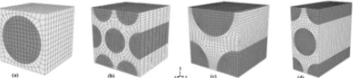
Two different unit cell configurations were used accordingly to the loading conditions and fiber arrangement. Thus square and hexagonal arrangements were applied for circular and square cross sections (cf. Figs. 4 and 5). The square arrangement was used for all loading conditions and the hexagonal arrangement was used to improve parallelism conditions representation.
In the finite element analysis, it was considered for active composite of circular cross-section fiber that the diameter is 1 mm, and for square cross-section fiber that the width is 1 mm. The fiber volume fraction is 55.5% of the unit cell total volume for both arrangements, that is, square and hexagonal, with circular or square fiber section (cf. Figs. 4 and 5).
quadratic piezoelectric brick elements (C3D20E–ABAQUSTM nomenclature for the element) with displacement degrees of freedom (DOF) and an additional electric potential DOF were used. These DOFs allow fully coupled electromechanical analyses.
Figure 4. Finite Element Models for circular section fiber: (a) square; (b) hexagonal; (c) hexagonal (shear 1-2) and (d) hexagonal (shear 2-3).
Figure 5. Finite Element Models for square section fiber: (a) square; (b) hexagonal; (c) hexagonal (shear 1-2) and (d) hexagonal (shear 2-3).
Material properties
The material properties related to the epoxy resin (composite matrix) and piezoelectric fiber (PZT-5A) were taken from Berger et al. (2005) and are shown in Table 1, according to orthotropic directions (coordinate system 1-2-3). For theses analyses presented, a fiber volume fraction of 55.5% for circular section, and also, for square section fiber was adopted and the fiber is oriented in direction 3.
Table 1. Material properties for fiber and matrix.
Fiber Matrix c11
GPa
121.0 3.86
c12 75.4 2.57
c13 75.2 2.57
c33 111.0 3.86
c44 21.1 0.64
c66 22.8 0.64
e13 C/m2
-5.4 -
e15 12.3 -
e33 15.8 -
ε 11
nF/m 8.11 0.0797
ε
33 7.35 0.0797
Boundary conditions
The simplified set of constitutive equations (cf. Eq. (2)), with prescribed boundary conditions allow the evaluation of the effective material properties. It is important to mention when the boundary conditions are applied in the RVE, more than one coefficient is obtained for each analysis. Therefore, to provide all eleven effective coefficients, only six analyses are necessary. More accurate results are obtained when loading is applied in fiber longitudinal direction, denoted here as z-direction (or direction 3), as well as x-direction and y-direction that are aligned with direction 1 and 2, respectively.
For the calculation of the effective coefficients c13eff and c33eff,
the boundary conditions applied on the RVE have admitted normal displacements set to zero on surfaces X+, X-, Y+ and Z- ( ̅11 = ̅22 =
̅
12 = ̅23 = ̅31 = 0), in accordance to the representation in Fig. 2.
Positive normal displacements have been prescribed on Z+ surface in z-direction ( ̅33≠ 0). Electrical potentials have been set to zero
on all surfaces ( 1 = 2 = 3 = 0). As only ̅33 is different from
zero, first and third lines of Eq. (2) can be used to obtain:
13 11/ 33,
eff
c =T S (10)
33 33/ 33.
eff
c =T S (11)
For the calculation of the effective coefficients e13eff, e33eff and
ε33eff, the RVE boundary conditions RVE have been zero for normal displacements on all surfaces ( ̅11 = ̅22 = ̅33 = ̅12 = ̅23 = ̅31 =
0), also. Electrical potential have been taken as zero on z-surface with respect to the Z+ surface. Therefore, from first, third, and last lines of Eq. (2), the effective values can be obtained as:
13 11/ 3,
eff
e =T E (12)
33 33/ 3,
eff
e = −T E (13)
33 3/ 3.
eff
D E
ε = (14) The effective coefficients c11eff and c12eff have been obtained
considering the RVE boundary conditions with similar conditions of those employed to the coefficients c13eff and c33eff, i.e. zero for
normal displacements on surfaces X-, Y+, Y-, Z+, and Z- ( ̅22 = ̅33
= ̅12 = ̅23 = ̅31 = 0). Positive displacements have been prescribed
on X+ surface in x-direction ( ̅11≠ 0). Electrical potentials have
been assumed zero on all surfaces ( 1 = 2 = 3 = 0). Because only
̅11 is different from zero, first and second lines of Eq. (2) can be used to obtain:
11 11/ 11,
eff
c =T S (15)
12 22/ 11.
eff
c =T S (16)
The effective coefficients ε11eff have been assessed with similar RVE boundary conditions of the effective coefficients e13eff, e33eff,
and ε33eff, which is zero for normal displacements on all surfaces ( ̅11 = ̅22 = ̅33 = ̅12 = ̅23 = ̅31 = 0). Null electrical potential on
X- surface applied to the X+ surface is considered. From the seventh line in Eq. (2), the effective value of the ε11eff coefficient can be given:
11 1/ 1.
eff
D E
ε = (17) For the calculation of the effective coefficients c66eff, the RVE
boundary conditions and loadings have admitted zero for displacements along z-direction on all nodes. All nodes located at the center line, that is perpendicular to the xy plane, had the displacements set to zero in x- and y-directions. Two opposite edges with nodes located at the cell border have been changed to cylindrical coordinate system and their displacements constrained, in order to avoid rigid body motion. Electrical potentials have been set to zero on all surfaces ( 1 = 2 = 3 = 0). Shear forces with
same modulus and opposite orientation have been applied on the surfaces Y+ and Y- in x-direction and on X+ and X- surfaces in y-direction, pursuing pure xy shear state. The parallelism conditions shown in Eqs. (8) and (9) must be applied between pair of surfaces
{ ̅} differs from zero. These boundary conditions are illustrated in Fig. 6(a). Therefore, from the fourth line in Eq. (2), it follows
66 12/ 12,
eff
c =T S (18)
Figure 6. Boundary conditions: (a) pure shear state in xy plane; (b) pure shear state in yz plane.
Finally, for the calculation of e15eff and c44eff coefficients, the
RVE boundary conditions (cf. in Fig. 6(b)) admit displacements in x-direction equal to zero for all nodes. Besides, all nodes located at the center line (perpendicular to the yz plane) present zero displacements in y- and z-directions. Similarly as in the case of the
c66efff coefficients, the two opposite edges with nodes located at the
cell border have been changed to cylindrical coordinate system and their displacements have been constrained to avoid rigid body rotation. Shear forces with same modulus and opposite orientation have been applied on the surfaces Y+ and Y- at z-direction and on
Z+ and Z- surfaces at y-direction, creating pure yz shear state. The conditions for parallelism, as shown by Eqs. (8) and (9), must be applied between pair of surfaces Z+ and Z-, and between Y+ and
Y-surfaces. These boundary conditions ensure the compatibility of the unit cell. Effective coefficient ε11eff has been determined from Eq. (17) and effective values for e15eff and c44eff can be obtained from the
fifth and eighth lines from Eq. (2), leading to:
(
)
15 2 11 2 / 23,
eff
e = − ⋅ +E ε D S (19)
(
)
44 23 2 15 / 23.
eff eff
c = T +E e⋅ S (20)
A computational procedure, based on Python language, has been developed to systematically calculate all RVE effective coefficients, thereby reducing exhaust manual work, saving time, and diminishing the chance of numerical errors. The code can also be used as template to evaluate piezoelectric fiber composites effective coefficients for arbitrary fiber volume fractions.
Results and Discussion
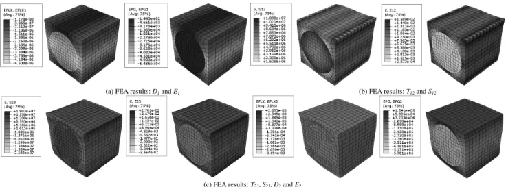
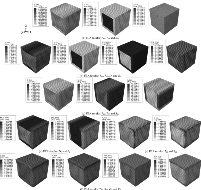
The effective coefficients for a piezoelectric circular cross section (PZT-5A) and epoxy resin matrix, typical for AFC arrangement, can be evaluated using results from Finite Element Analysis (FEA) and their set of equations are shown in Eq. (5). As observed in Fig. 7 and Fig. 8, it is possible to assess the numerical results to calculate the parameters required by Eq. (5).
(a) FEA results: T11, T33 and S33
(b) FEA results: T11, T33, D3 and E3
(c) FEA results: T11, T22 and S11
J. of the Braz. Soc. of Mech. Sci. & Eng. Copyright 2012 by ABCM Special Issue 2012, Vol. XXXIV / 367
(a) FEA results: D1 and E1 (b) FEA results: T12 and S12
(c) FEA results: T23, S23, D2 and E2
Figure 8. Square arrangement with circular geometry: non-zero average fields for 4th, 5th and 6th analyses.
It is worth remembering that all 11 effective coefficients (cf.
Eq. (2)) have been calculated for one specific fiber volume fraction, that is, 55.5%. The method is applied and the results are compared with analytical and numerical results available in the technical literature by Berger et al. (2005) and Moreno et al. (2009), respectively. The results are summarized in Table 2. The column assigned as (1) refers to results obtained by Berger et al. (2005), while columns (2) and (3) refer to results obtained by Moreno et al. (2009). The column (1) by Berger et al. (2005) is related to analytical formulation achieved with an asymptotic homogenization method (AHM) for circular cross section. The columns (2) and (3) summarize the coefficients obtained by Moreno et al. (2009) using FEA for circular cross section with square and hexagonal unit cell arrangement, respectively.
The columns (4) and (5) summarize the effective coefficients computed by the method proposed in this work, admitting circular cross section for square and hexagonal unit cell arrangement, respectively. The effective coefficient difference values (∆) between results are presented in the last four columns of Table 2. The first and second columns, denoting the difference values ∆1 and ∆2, respectively, are taken from the analytical and numerical results presented by Berger et al. (2005) and Moreno et al. (2009) for square and hexagonal arrangements, respectively. The third and fourth columns, denoting the difference values ∆3 and ∆4, respectively, are related to the analytical formulation by Berger et al. (2005) and the present work for square and hexagonal unit cell arrangements, respectively.
Table 2. Effective properties of circular cross section for square and hexagonal unit cell arrangement.
Coeff. Units AHM (1)
Ansys (2)
Ansys (3)
Abaqus (4)
Abaqus
(5) ∆∆∆∆1[%] ∆∆∆∆2 [%] ∆∆∆∆3 [%] ∆∆∆∆4 [%]
c11eff
GPa
9.5 10.88 10.68 10.856 10.356 14.53 12.42 14.27 9.01
c12eff 5.6 4.65 5.22 4.666 4.955 16.96 6.79 16.68 11.52
c13eff 6.0 6.04 6.19 6.043 6.235 0.67 3.17 0.72 3.92
c33eff 35.0 35.25 35.21 35.130 36.919 0.71 0.60 0.37 5.48
c44eff 2.2 2.15 1.95 1.969 1.905 2.27 11.36 10.50 13.41
c66eff 2.0 1.54 1.81 1.536 1.841 23.00 9.50 23.20 7.93
e13eff
C/m2
-0.26 -0.258 -0.269 -0.2584 -0.2633 0.77 3.46 0.62 1.27
e15eff 0.02 0.0241 0.0164 0.0195 0.0201 20.50 18.00 2.50 0.50
e33eff 11.0 10.860 10.86 10.8642 11.0106 1.27 1.27 1.23 0.10
ε11eff
nF/m 0.28 0.284 0.303 0.2867 0.3026 1.43 8.21 2.39 8.07
ε
33eff 4.2 4.270 4.27 4.2704 4.3222 1.67 1.67 1.68 2.91
∆1 - Comparing (1) and (2): Berger et al. (2005) × Moreno et al. (2009) (Square Unit Cell)
∆2 - Comparing (1) and (2): Berger et al. (2005) × Moreno et al. (2009) (Hexagonal Unit Cell)
∆3 - Comparing (1) and (3): Berger et al. (2005) × Present work (Square Unit Cell)
As shown in Table 2, the effective coefficients with major difference between the analytical and numerical approach of this work have been c11eff, c12eff, c66eff, and e15eff for square cell. Similarly
these differing results for those coefficients were also stated by other authors (Berger et al., 2005; Kar-Gupta and Venkatesh, 2005, 2007; Moreno et al., 2009). These coefficients are mainly influenced by the composite transversal behavior. Other influence is observed for the effective coefficients values obtained from the hexagonal cell, which can be related to the loading application. In quadratic cell, mechanical loading is applied through the epoxy resin matrix, while in the hexagonal cell arrangement it has been applied through both epoxy matrix and piezoelectric fiber.
In a hexagonal fiber arrangement, it is well known that the transverse isotropy is fully accomplished, resulting in approximate values for those found analytically. Several hypotheses can be adopted to illustrate the composites crystal symmetry, thereby creating a variety of combinations for matrix and fiber constituents
with varying degrees of anisotropy. Here, transversely isotropic piezo-fiber (poled along direction 3) and isotropic matrix (passive behavior) have been adopted, consequently the result for this combination leads to a transversely isotropic RVE behavior (poled along direction 3). Due to the crystal system tetragonal (square cell) presenting 4 mm symmetry and the crystal system hexagonal (hexagonal cell) with 6 mm symmetry, the constitutive model has shown better effective coefficient predictions for hexagonal than square cell arrangement.
On the other hand, the model is highly influenced by the applied RVE boundary conditions, due to the fact that values are in the order of Giga and Nano. For that reason, the model can be highly sensitive to changes in boundary conditions. For the remaining effective coefficients, the method applied to square and hexagonal RVE arrangements has shown adequate agreement with those presented by asymptotic homogenization method (Berger et al., 2005).
(a) FEA results: T11, T33 and S33
(b) FEA results: T11, T33, D3 and E3
(c) FEA results: T11, T22 and S11
(d) FEA results: D1 and E1 (e) FEA results: T12 and S12
(f) FEA results: T23, S23, D2 and E2
J. of the Braz. Soc. of Mech. Sci. & Eng. Copyright 2012 by ABCM Special Issue 2012, Vol. XXXIV / 369
As commented earlier, present investigation has also considered other piezoelectric fiber cross-sectional geometry, that is, a square. Analogously to the previous investigation, the RVE corresponds to the piezoelectric fiber and an epoxy resin matrix with volume fiber fraction of 55.5%. Thus, all 11 effective coefficients for a square cross section can be evaluated using FEA and subsequent application of the method proposal. Figure 9 presents FEA results for aforementioned boundary conditions and respective loading described earlier.
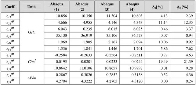
Table 3 presents results related to the homogenized properties and comparisons between both circular and square cross sections, admitting square and hexagonal unit cells. The columns (1) to (4) present the coefficients obtained by the proposed method of this work. Differently from the previous results for circular piezoelectric fiber (cf. Table 2), here no analytical predictions have been available
to serve as comparison basis. For this reason, the comparisons have been made only for the numerical analyses as explained in this work for circular and square cross sections.
The columns (1) and (2) have the coefficients for circular cross section (square and hexagonal unit cells, respectively), while the columns (3) and (4) have effective coefficients for square cross section (also for square and hexagonal unit cells, respectively). The values attained are compared between results for circular and square piezoelectric fiber cross section, and the differences ∆1 and ∆2 (percentage) between these results is presented in the last two columns of Table 3. The difference ∆1 is taken between results for circular and square cross sections, adopting square unit cell, while ∆2 considers the difference between results for circular and square geometries, respectively, for hexagonal RVE.
Table 3. Effective properties for square cross section for square and hexagonal unit cell arrangement.
Coeff. Units Abaqus (1)
Abaqus (2)
Abaqus (3)
Abaqus
(4) ∆∆∆∆1[%] ∆∆∆∆2 [%]
c11eff
GPa
10.856 10.356 11.304 10.603 4.13 2.39
c12eff 4.666 4.955 4.146 4.343 11.14 12.35
c13eff 6.043 6.235 6.015 6.025 0.46 3.37
c33eff 35.130 36.919 35.106 36.573 0.07 0.94
c44eff 1.969 1.905 2.167 2.094 10.06 9.92
c66eff 1.536 1.841 1.446 1.701 5.86 7.62
e13eff
C/m2
-0.2584 -0.2633 -0.2564 -0.2511 0.77 4.63
e15eff 0.0195 0.0201 0.0233 0.0244 19.49 21.39
e33
eff
10.8642 11.0106 10.8657 10.9798 0.01 0.28
ε11eff
nF/m 0.2867 0.3026 0.2852 0.3158 0.52 4.36
ε
33eff 4.2704 4.3222 4.2705 4.3120 0.00 0.24
∆1 -Comparing (1) and (3): Circular fiber cross section (square RVE) × Square fiber cross section (square RVE)
∆2 -Comparing (2) and (4): Circular fiber cross section (hexagonal RVE) × Square fiber cross section (hexagonal RVE)
As shown in Table 3, the effective coefficients for both square and hexagonal unit cells (volumetric fraction of 55.5%) have provided small difference values. However, as in previous comparisons, the c12eff, c66eff and e15eff coefficients have shown
significant differences for both square and hexagonal unit cells, due to the aspects previously discussed for the circular cross-section piezo-fiber case (cf. Table 2). Besides, the geometries of fiber cross section are different.
Conclusions
The method proposal based on representative volume element (RVE) for predicting the homogenized properties of piezoelectric fiber composites using the finite element analysis (FEA) has shown adequate results. Longitudinal and transversal elastic and piezoelectric effective coefficients for a piezo-ceramic fiber with circular geometry embedded in a non-piezoelectric material (epoxy resin matrix) have been evaluated and compared to analytical solutions based on the asymptotic homogenization method (Berger et al., 2005). The method uses Python programming language to impose boundary conditions automatically, which speeds up considerably the calculations. This approach, however, requires particular care with RVE boundary conditions. If the boundary conditions are not applied correctly, then rigid body motions may occur and contaminate the numerical calculations. Although, great
amount of boundary conditions may lead to over constrained RVE, thereby affecting the model, also. Therefore, it is very important to balance the boundary conditions application.
In fact, numerical results in this investigation, for the square arrangement of fibers with circular geometry, have shown to be similar to those encountered in the literature. However, when comparing AFC circular and square cross-section active composites, the predicted coefficients difference values have shown that this method has appropriate convergence. These outcomes allow inferring that the method proposal is adequate to estimate effective properties for active composites.
Finally, the achievements of this investigation have also allowed concluding that the elastic transversely isotropic behavior, piezoelectric activity of the constituent phases, and influence of the relative orientation of the fiber and matrix poling directions in the hexagonal RVE arrangements provide better results when comparing with analytical ones. The reason for that can be related to the piezo-fiber crystal arrangement. Therefore, the determination of effective coefficients needs to be checked using experimental and/or other analytical analyses.
Acknowledgements
and FAPEMIG for partially funding the present research work through the INCT-EIE. The authors also would like to thank Prof. Reginaldo Teixeira Coelho (EESC-USP) for the ABAQUSTM license.
References
Abaqus, 2010, “Documentation”, Version 6.10-1, Dassault Systèmes, United States of America.
Azzouz, M.S., Mei, C., Bevan, J.S. and Ro, J.J., 2001, “Finite element modeling of MFC/AFC actuators and performance of MFC”, Journal of Intelligent Material Systems and Structures, Vol. 12, pp. 601-612.
Bent, A.A. and Hagood, N.W., 1993b “Development of Piezoelectric Fiber Composites for Structural Actuation,” Proceeding of the 34th AIAA/ASME/ASCE/AHS Structures, Structural Dynamics and Materials Conference, April, La Jolla, CA, AIAA Paper No. 93-1717-CP pp. 3625-3638.
Bent, A.A., 1997, “Active fiber composites for structural actuation”, Thesis (PhD), Department of Aeronautics and Astronautics, Massachusetts Institute of Technology, 209 p.
Berger, H., Kari, S., Gabbert, U., Rodriguez-Ramos, R., Guinovart, R., Otero, J.A. and Bravo-Castillero, J., 2005, “An analytical and numerical approach for calculating effective material coefficients of piezoelectric fiber composites”, International Journal of Solids and Structures, Vol. 42, pp. 5692-5714.
Berger, H., Kari, S., Gabbert, U., Rodriguez-Ramos, R., Bravo-Castillero, J., Guinovart-Diaz, R., Sabina, F.J. and Maugin, G.A., 2006, “Unit cell models of piezoelectric fiber composites for numerical and analytical calculation of effective properties”, Smart Materials and Structures, Vol. 15, pp. 451-458.
Bravo-Castillero, J., Guinovart-Diaz, R., Sabina, F.J. and Rodríguez-Ramos, R., 2001, “Closed form expressions for the effective coefficients of a fiber-reinforced composite with transversely isotropic constituents – II. Piezoelectric and square symmetry”, Mechanics of Materials, Vol. 33, pp. 237-248.
Chan, H.L.W. and Unsworth, J., 1989, “Simple model for piezoelectric ceramic/polymer 1-3 composites used in ultrasonic transducer applications”,
IEEE Transactions on Ultrasonics, Ferroelectrics and Frequency Control, Vol. 36, pp. 434-441.
Dunn, M.L. and Taya, M., 1993, “Micromechanics predictions of the effective electroelastic moduli of piezoelectric composites”, International Journal of Solids and Structures, Vol. 30, pp. 161-175.
Gaudenzi, P., 1997, “On the electro mechanical response of active composite materials with piezoelectric inclusions”, Computers & Structures, Vol. 65, pp. 157-168.
Kar-Gupta, R. and Venkatesh, T.A., 2005, “Electromechanical response of 1-3 piezoelectric composites: effect of poling characteristics”, Journal of Applied Physics, Vol. 98, 14 p.
Kar-Gupta, R. and Venkatesh, T.A., 2007, “Electromechanical response of 1-3 piezoelectric composites: a numerical model to assess the effects of fiber distribution”, Acta Materialia, Vol. 55, pp. 1275-1292.
Moreno, M.E., Tita, V. and Marques, F.D., 2009, “Finite element analysis applied to evaluation of effective material coefficients for piezoelectric fiber composites”, in 2009 Brazilian Symposium on Aerospace Eng. & Applications, September 14-16, 2009, S. J. Campos, SP, Brazil.
Moreno, M.E., Tita, V. and Marques, F.D., 2010, “Influence of boundary conditions on the determination of effective material properties for active fiber composites”, in 2010 Pan-American Congress of Applied Mechanics, January 04-08, 2010, Foz do Iguaçu, PR, Brazil.
Paradies, R. and Melnykowycz, M., 2007, “Numerical stress investigation for piezoelectric elements with circular cross section and interdigitated electrodes”, Journal of Intelligent Material Systems and Structures, Vol. 18, pp. 963-972.
Pérez-Fernandez, D., 2009, “Un enfoque integrador de métodos asintóticos y variacionales para la evaluación del comportamiento efectivo de materiales compuestos magneto-electro-elásticos no lineales provistos de una estructura periódica.”, Tesis (Doctor en Ciencias Matemáticas) – Instituto de Cibernética, Matemática y Física, Departamento de Física Aplicada, La Habana, Cuba.
Pettermann, H.E. and Suresh, S., 2000, “A comprehensive unit cell model: a study of coupled effects in piezoelectric 1-3 composites”,
International Journal of Solids and Structures, Vol. 37, pp. 5447-5464. Piezoelectric Ceramic for Sonar Transducers (Hydrophones & Projectors) Military Standard US DOD MIL STD 1376 A (SH) (1984).
Poizat, C. and Sester, M., 1999, “Effective properties of composites with embedded piezoelectric fibres”, Computational Materials Science, Vol. 16, pp. 89-97.
Rodríguez-Ramos, R., Sabina, F.J., Guinovart-Díaz, R. and Bravo-Castillero, J., 2001, “Closed form expressions for the effective coefficients of a fiber-reinforced composite with transversely isotropic constituents – I. Elastic and square symmetry”, Mechanics of Materials, Vol. 33, pp. 223-235.
Smith, W.A. and Auld, B.A., 1991, “Modeling 1-3 composite-piezoelectrics: thickness-mode oscillations”, IEEE Transactions on Ultrasonics, Ferroelectrics and Frequency Control, Vol. 38, pp. 40-47.
Tan, X.G. and Vu-Quoc, L., 2005, “Optimal solid shell element for large deformable composite structures with piezoelectric layers and active vibration control”, International Journal for Numerical Methods in Engineering, Vol. 64, pp. 1981-2013.