Mapping CH<sub>4</sub> : CO<sub>2</sub> ratios in Los Angeles with CLARS-FTS from Mount Wilson, California

(1)

ACPD

14, 17037–17066, 2014

Mapping CH4: CO2

ratios in Los Angeles with CLARS-FTS from Mount Wilson,

California

K. W. Wong et al.

Title Page

Abstract Introduction

Conclusions References

Tables Figures

◭ ◮

Back Close

Full Screen / Esc

Printer-friendly Version Interactive Discussion

Discussion

P

a

per

|

Discus

sion

P

a

per

|

Discussion

P

a

per

|

Discussion

P

a

per

|

Atmos. Chem. Phys. Discuss., 14, 17037–17066, 2014 www.atmos-chem-phys-discuss.net/14/17037/2014/ doi:10.5194/acpd-14-17037-2014

This discussion paper is/has been under review for the journal Atmospheric Chemistry and Physics (ACP). Please refer to the corresponding final paper in ACP if available.

Mapping CH

₄

: CO

₂

ratios in Los Angeles

with CLARS-FTS from Mount Wilson,

California

K. W. Wong1, D. Fu1, T. J. Pongetti1, S. Newman2, E. A. Kort4, R. Duren1,

Y.-K. Hsu3, C. E. Miller1, Y. L. Yung2, and S. P. Sander1

1

NASA Jet Propulsion Laboratory, Pasadena, California, USA

2

California Institute of Technology, Pasadena, California, USA

3

California Air Resources Board, Sacramento, California, USA

4

University of Michigan, Ann Arbor, Michigan, USA

Received: 23 May 2014 – Accepted: 8 June 2014 – Published: 26 June 2014

Correspondence to: K. W. Wong (clare.wong@jpl.nasa.gov)

(2)

ACPD

14, 17037–17066, 2014

California

K. W. Wong et al.

Title Page

Tables Figures

◭ ◮

Back Close

Full Screen / Esc

Discussion

P

a

per

|

Discus

sion

P

a

per

|

Discussion

P

a

per

|

Discussion

P

a

per

|

Abstract

The Los Angeles megacity, which is home to more than 40 % of the population in California, is the second largest megacity in the United States and an intense source of anthropogenic greenhouse gases (GHGs). Quantifying GHG emissions from the megacity and monitoring their spatiotemporal trends are essential to be able to

un-5

derstand the effectiveness of emission control policies. Here we measure carbon

diox-ide (CO₂) and methane (CH₄) across the Los Angeles megacity using a novel

ap-proach – ground-based remote sensing from a mountaintop site. A Fourier Transform Spectrometer (FTS) with agile pointing optics, located on Mount Wilson at 1.67 km

above sea level, measures reflected near infrared sunlight from 29 different surface

10

targets on Mount Wilson and in the Los Angeles megacity to retrieve the slant

col-umn abundances of CO2, CH4 and other trace gases above and below Mount

Wil-son. This technique provides persistent space and time resolved observations of path-averaged dry-air GHG concentrations, XGHG, in the Los Angeles megacity and sim-ulates observations from a geostationary satellite. In this study, we combined high

15

sensitivity measurements from the FTS and the panorama from Mount Wilson to

characterize anthropogenic CH4 emissions in the megacity using tracer : tracer

cor-relations. During the period between September 2011 and October 2013, the

ob-served XCH₄: XCO₂ excess ratio, assigned to anthropogenic activities, varied from

5.4 to 7.3 ppb CH₄(ppm CO₂)−1, with an average of 6.4±0.5 ppb CH₄(ppm CO₂)−1

20

compared to the value of 4.6±0.9 ppb CH4(ppm CO2)

−1

expected from the Califor-nia Air Resources Board (CARB) bottom-up emission inventory. Persistent elevated

XCH₄: XCO₂excess ratios were observed in Pasadena and in the eastern Los Angeles

megacity. Using the FTS observations on Mount Wilson and the bottom-up CO2

emis-sion inventory, we derived a top-down CH4emission of 0.39±0.06 Tg CH4year−

1 in the

25

Los Angeles megacity. This is 18–61 % larger than the state government’s bottom-up

(3)

ACPD

14, 17037–17066, 2014

California

K. W. Wong et al.

Title Page

Tables Figures

◭ ◮

Back Close

Full Screen / Esc

Discussion

P

a

per

|

Discus

sion

P

a

per

|

Discussion

P

a

per

|

Discussion

P

a

per

|

1 Introduction

The Los Angeles megacity – a sprawling urban expanse of ∼100 km×100 km and

15 million people – covers only∼4 % of California’s land area but is home to more than

43 % of its population and dominates the state’s anthropogenic greenhouse gas (GHG)

emissions. By treating the megacity as an effective “point source”, we can quantify

5

trends in this critical component of the state’s GHG emissions and support California’s goal of reducing GHG emissions to the 1990 level by 2020 mandated by the state’s The Global Warming Solutions Act of 2006 (AB32).

Emissions of carbon dioxide (CO2) and methane (CH4) in the Los Angeles megacity

originate largely from different economic sectors and are expected to have distinctly

dif-10

ferent spatial and temporal patterns. Anthropogenic CO2is derived mainly from motor

vehicle exhaust (Transportation), exhibiting strong diurnal variability and weak seasonal variability, and from natural gas fueled power plants (Power) with a few large stationary

emitters and significant seasonal variability. Overall CO2 emissions for transportation

and power plants are known to within±10 % from fuel usage and emission factors. On

15

the other hand, the CH₄emissions budget is highly uncertain and contains significant

but poorly quantified emissions from a variety of sources such as landfills and wastew-ater treatment plants (Waste), oil and gas production, storage and delivery infrastruc-ture (Power and Residential), dairy farms (Agriculinfrastruc-ture) and geologic seeps (Geology).

Recent studies estimating CH4emissions from atmospheric observations have shown

20

that the bottom-up total CH4emissions inventory in the Los Angeles megacity have

un-certainties of 30 % to>100 % (Wunch et al., 2009; Hsu et al., 2010; Wennberg et al.,

2012; Jeong et al., 2013; Peischl et al., 2013). Atmospheric observations may be used

to characterize spatial and temporal patterns in CO2 and CH4 within the Los Angeles

megacity and to provide initial estimates of sectoral emissions attribution.

25

(4)

ACPD

14, 17037–17066, 2014

California

K. W. Wong et al.

Title Page

Tables Figures

◭ ◮

Back Close

Full Screen / Esc

Discussion

P

a

per

|

Discus

sion

P

a

per

|

Discussion

P

a

per

|

Discussion

P

a

per

|

measurements are relatively insensitive to boundary layer height variations and are less influenced by local sources than ground in situ measurements, they should be

more representative of the area. They reported that the bottom-up CH4 emissions for

the Los Angeles megacity are less than half of the top-down CH4emissions. The large

uncertainty in the bottom-up CH₄emission inventory in the Los Angeles megacity has

5

also been supported by the CH4: CO2ratios observed by aircraft campaigns,

ARCTAS-CARB in 2008 and CalNex in 2010 (Wennberg et al., 2012; Peischl et al., 2013), and in-situ observations on Mount Wilson (Hsu et al., 2010).

Despite the potential of atmospheric observations to quantify the emissions of CH₄,

CO2 and other GHGs in the Los Angeles megacity, they have certain limitations for

10

tracking long-term GHG emissions. Kort et al. (2013) showed that surface in situ ob-servations from no single site within or adjacent to the Los Angeles megacity accu-rately capture the emissions from the entire region. Similarly, ground-based total col-umn measurements from Pasadena also lack sensitivity to emissions from across the entire region. Kort et al. (2013) concluded that the size and complexity of the Los

An-15

geles megacity urban dome requires a network of at least eight strategically located continuous surface in situ observing sites to quantify and track GHG emissions over time. However, this minimum network would have limited capabilities to identify and isolate emissions from specific sectors and/or localized sources. It is therefore neces-sary to develop a robust, long-term measurement solution, which resolves emissions

20

the Los Angeles megacity both spatially and temporally.

The present study reports GHG measurements of the Los Angeles megacity from an elevated vantage point, the California Laboratory for Atmospheric Remote Sens-ing (CLARS), located on Mt Wilson 1670 m a.s.l. and overlookSens-ing the Los Angeles

megacity (Fig. 1). We present column averaged dry air mole fraction CO2 (XCO2)

25

and CH4 (XCH4) measurements for 29 reflection points distributed across Los

An-geles. The measurements cover daylight hours for the two-year period between

2011 and 2013. We determine the enhancements in XCH4 and XCO2 in the basin

(5)

ACPD

14, 17037–17066, 2014

California

K. W. Wong et al.

Title Page

Tables Figures

◭ ◮

Back Close

Full Screen / Esc

Discussion

P

a

per

|

Discus

sion

P

a

per

|

Discussion

P

a

per

|

Discussion

P

a

per

|

XCH₄(excess) : XCO₂(excess) ratio to quantify emissions in the megacity. We compare

our results to column, surface in-situ and aircraft in situ observations and compare our

derived megacity CH4emissions estimates with the results from previous studies.

CLARS provides a unique long-term data record that simulates geostationary (GEO) satellite observations for the Los Angeles basin. CLARS maps the diurnal variability

5

of both XCO2 and XCH4 within the Los Angeles urban dome with hourly time scales.

It has functioned operationally since 2011, and its sustained measurements are yield-ing insights into the scientific value of GEO GHG monitoryield-ing, as well as helpyield-ing to define GEO-based GHG measurement requirements. Existing and future satellite in-struments such as TES (AURA), TANSO-FTS (GOSAT), and OCO-2, all sample from

10

sun-synchronous low-earth orbits. These platforms sample globally, but return to the same measurement point on the Earth infrequently, with repeat cycles ranging from days to weeks. In contrast, GEO measurements, such as those from the proposed Geostationary Fourier Transform Spectrometer (GEO-FTS), map the complete field of regard with high spatial resolution (<10 km horizontal resolution) many times per day

15

(Key et al., 2012). Measurements from a mountaintop location, such as CLARS, pro-vide similar spatial and temporal resolution as GEO measurements but with a larger viewing zenith angle which enhances the optical path in the planetary boundary layer.

We also demonstrate simultaneous XCH4 and XCO2 measurements are essential to

quantify megacity GHG emissions and also provide critical information from which to

20

attribute emissions to different economic sectors.

2 Measurement technique

2.1 CLARS-FTS

A JPL-built Fourier Transform Spectrometer (FTS) has been deployed since 2010 at the CLARS facility on Mount Wilson at an altitude of 1670 m a.s.l. overlooking the Los

25

(6)

ACPD

14, 17037–17066, 2014

California

K. W. Wong et al.

Title Page

Tables Figures

◭ ◮

Back Close

Full Screen / Esc

Discussion

P

a

per

|

Discus

sion

P

a

per

|

Discussion

P

a

per

|

Discussion

P

a

per

|

Observations (SVO) and the Los Angeles Basin Surveys (LABS). In the SVO mode,

the FTS points at a Spectralon® plate placed immediately below the FTS telescope

to quantify the total column CO2and CH4above the megacity (above 1670 m and the

basin planetary boundary layer (PBL) height). The SVO measurements represent ap-proximately free tropospheric background levels. In the LABS mode, the FTS points

5

downward at 28 geographical points in the basin acquiring spectra from reflected sun-light in the near-infrared region (Table 1). Our measurement technique from Mount Wilson mimics satellite observations, which measure surface reflectance from space or atmospheric absorptions of GHGs along the optical path – (1) from the sun to the surface and (2) from the surface to the instrument. The locations of the reflection points

10

are selected to provide the best coverage of the megacity (Fig. 1). In addition, reflec-tion points are chosen with uniform surface albedo across the spectrometer field of view using a near infrared camera. Reflection points sample from the San Bernardino Mountains in the east to the Pacific coast in the west, and from the base of the San Gabriel Mountains in the north to Long Beach Harbor and Orange County in the south.

15

For a typical PBL height, the geometric slant paths within the PBL range from∼4 km

(Santa Anita Park) to∼39 km (Lake Mathews). The points in Table 1 are the baseline

raster pattern, but can be modified easily if desired. In the standard measurement cy-cle, the FTS points at these 28 reflection points and performs four SVO measurements per cycle. There are 5–8 measurement cycles per day depending on the time of the

20

year.

The spectral resolution used in the CLARS-FTS measurement is 0.12 cm−1, with an

angular radius of the field of view of 0.5 mrad. The footprints in the Los Angeles basin

are ellipses with surface areas ranging from 0.04 to 21.62 km2 (Table 1). The

point-ing calibration procedure is designed to maximize pointpoint-ing accuracy (Fu et al., 2014).

25

Pointing uncertainties are primarily due to errors arising from gimbal tilt and minor position-dependent flexing of the pointing system structure. After pointing calibration corrections are applied, the CLARS-FTS pointing system has a total uncertainty of

(7)

ACPD

14, 17037–17066, 2014

California

K. W. Wong et al.

Title Page

Tables Figures

◭ ◮

Back Close

Full Screen / Esc

Discussion

P

a

per

|

Discus

sion

P

a

per

|

Discussion

P

a

per

|

Discussion

P

a

per

|

results in a ground distance error of about 60 m for a reflection point located 20 km from

Mount Wilson. Uncertainty is 0.045◦ (1 sigma) in elevation, that is, 8 % of the

CLARS-FTS field of view, resulting in a ground distance error of about 16 m for a target that is 20 km from Mount Wilson. Details concerning the CLARS-FTS design, operation and calibration are described in Fu et al. (2014).

5

2.2 Data processing

The CLARS interferogram processing program (CLARS-IPP) converts the recorded in-terferograms into spectra. The CLARS-IPP also corrects for solar intensity variations and phase error. 12 single scan spectra are co-added over a period of 3 min for each

reflection point to achieve a spectral signal-to-noise ratio (SNR) of∼300 : 1 for LABS

10

measurements and∼450 : 1 for SVO measurements. The instrument line shape (ILS)

of the CLARS-FTS is characterized using an external lamp and an HCl gas cell. Our experiment works on a simple Beer-Lambert principle where the number densities of

CO₂and CH₄are proportional to the optical depths measured for rotationally resolved

near infrared absorption spectra. Slant column density (SCD), the total number of

ab-15

sorbing molecule per unit area along the sun-Earth-instrument optical path, is retrieved

for CO₂and CH₄using a modified version of the GFIT algorithm (Wunch et al., 2011; Fu

et al., 2014). Descriptions of the CLARS-FTS data processing and retrieval algorithm

are included in Fu et al. (2014). In the present analysis, we retrieve CO2from bands at

1.6 µm, CH4at 1.67 µm, and O2at 1.27 µm. The retrieved SCDs are converted to slant

20

column-averaged dry air mole fractions, XCO₂ and XCH₄, by normalizing to SCD_O

2 (Eq. 1).

XGHG=SCDGHG

SCD_O

2

×0.2095 (1)

This method has been shown to improve the precision of XCO₂ and XCH₄ retrievals

since SCDO₂ retrieval effectively cancels out first-order path length, instrumental, and

(8)

ACPD

14, 17037–17066, 2014

California

K. W. Wong et al.

Title Page

Tables Figures

◭ ◮

Back Close

Full Screen / Esc

Discussion

P

a

per

|

Discus

sion

P

a

per

|

Discussion

P

a

per

|

Discussion

P

a

per

|

retrieval algorithm errors (Washenfelder and Wennberg, 2003; Washenfelder et al., 2006; Wunch et al., 2011; Fu et al., 2014). Measurement precisions are 0.3 ppm

for XCO2 (∼0.1 %) and 2.5 ppb for XCH4 (∼0.1 %) for the SVO measurements and

0.6 ppm for XCO₂ (∼0.1 %) and 4.7 ppb for XCH₄ (∼0.2 %) for the LABS

measure-ments. Estimated measurement accuracies are <_{3.1 % for XCO}₂ _and <_{6.0 % for}

5

XCH4, driven mainly by uncertainties in laboratory spectra line parameters.

2.3 Data filtering

Poor air quality in Los Angeles causes visibility reduction due to aerosol scattering. While the impact of aerosol scattering is significantly lower in the infrared than the visible and ultraviolet spectral regions, CLARS-FTS trace gas retrievals can be affected

10

by aerosols due to the long optical path length in the boundary layer. In addition to

aerosol, the Los Angeles megacity is often affected by morning marine layer fog and

low clouds, which influence the data quality.

Individual retrievals are analyzed with multiple post-processing filters to ensure data

quality, similar to the QA/QC filters adopted in the Atmospheric CO2observations from

15

Space (ACOS) – GOSAT data processing (O’Dell et al., 2012; Crisp et al., 2012; Man-drake et al., 2013). Table 2 summarizes the filtering criteria. Data with poor spectral fitting quality, such as with large solar zenith angle (SZA), low SNR and/or large fit-ting residual root mean square errors (RMS), are removed. Data are also screened for clouds and aerosols using the ratio of retrieved to geometric oxygen SCDs as the

20

criterion. The geometric oxygen SCD is calculated using surface pressure from Na-tional Center for Environmental Prediction (NCEP) reanalysis data assuming hydro-static equilibrium, a constant oxygen dry-air volume mixing ratio of 0.2095 along the optical path and no scattering or absorption occurs (Fu et al., 2014). Because oxygen is well mixed in the atmosphere, deviations in the retrieved oxygen SCD from the

geomet-25

ric oxygen SCD indicate variations of the light path due to clouds and/or aerosols, as-suming deviations are larger than the retrieval uncertainty, that is,<0.3 % for SVO

(9)

ACPD

14, 17037–17066, 2014

California

K. W. Wong et al.

Title Page

Tables Figures

◭ ◮

Back Close

Full Screen / Esc

Discussion

P

a

per

|

Discus

sion

P

a

per

|

Discussion

P

a

per

|

Discussion

P

a

per

|

high clouds, data are filtered out when the corresponding SVO oxygen SCD ratio is less than 1 or greater than 1.1. For low clouds, data with retrieved target oxygen SCD devi-ating more than 10 % from the geometric value are removed. We use the same criteria to take out data with heavy aerosol loading which leads to significant modification in the light path. This filtering approach is equivalent to that used by ACOS, which compares

5

the retrieved surface pressure to reanalysis data (O’Dell et al., 2012). As a result of our data filters, more data are removed for reflection points located further away from Mount Wilson since these measurements have larger fractions of their optical paths in the PBL and are more likely to encounter substantial scattering (Fig. 2).

Numerous studies have shown that aerosol scattering the atmosphere has an impact

10

on the retrieved trace gas mixing ratios from space-based observations in the near-infrared (Aben et al., 2007; Yoshida et al., 2011; Crisp et al., 2012). Zhang et al. (2014) used a numerical two-stream radiative transfer model (RTM) validated against the VLI-DORT full-physics RTM (Spurr et al., 2006) to estimate the expected biases in the

retrieved values of XCO2 and XCH4 from CLARS observations. The model was used

15

to set the value for the CLARS aerosol filter criterion in terms of the ratio of measured to geometric optical path length derived from the 1.27 µm absorption band of molecular oxygen (see section 4.1).

3 Observations

3.1 Diurnal variations of XCO2and XCH4: SVO vs. LABS

20

Due to the difference in the measurement geometry between the SVO mode and the

LABS mode, the diurnal patterns of XCO2and XCH4differ significantly. Figure 3 shows

an example of the diurnal variations of raw and filtered XCO2and XCH4measurements

for the SVO mode, and the LABS west Pasadena and Santa Anita Park targets from

∼08:30 to∼16:30 LT on seven continuous days during the period 5–11 May 2012. The

25

(10)

ACPD

14, 17037–17066, 2014

California

K. W. Wong et al.

Title Page

Tables Figures

◭ ◮

Back Close

Full Screen / Esc

Discussion

P

a

per

|

Discus

sion

P

a

per

|

Discussion

P

a

per

|

Discussion

P

a

per

|

and 1700 ppb XCH₄ during this period. The constant diurnal pattern was observed

because the FTS is located most of the time above the planetary boundary layer where sources are located (Newman et al., 2013). Therefore the SVO measurements do not

capture variations of atmospheric CO₂ and CH₄ mixing ratio due to emissions in the

Los Angeles megacity.

5

On the other hand, the west Pasadena and Santa Anita Park reflection points

exhib-ited strong diurnal signals in XCO₂ and XCH₄, with a minimum typically in the early

morning of around 405–410 ppm for XCO2 and 1800–1900 ppb for XCH4 and a

max-imum of up to 420 ppm for XCO2 and 1950 ppb for XCH4 at noon or in the early

af-ternoon. Variability in CO₂ and CH₄ emissions and atmospheric transport resulted in

10

daily ranges of variation of 10–30 ppm XCO₂and 100–200 ppb XCH₄during the period

of 5–11 May 2012. With a typical boundary layer height, the west Pasadena and the Santa Anita Park measurements sample horizontally over a few kilometers in the PBL

and are therefore sensitive to emission signatures. The buildup of XCO₂and XCH₄ in

the morning and the falloffin the afternoon are due to a combination of accumulation of

15

emissions and dilution/advection processes in basin. Similar diurnal patterns of XCO2

and XCH₄(that is, peak at noon or early afternoon) have been observed in Pasadena

by a TCCON station (Wunch et al., 2009). However, the column enhancements

ob-served by TCCON are typically less than 2–3 ppm in XCO2 and 20–40 ppb in XCH4.

These enhancements are significantly smaller than those derived from the

CLARS-20

FTS measurements which have a longer optical path within the PBL compared with TCCON at the same SZA.

Variations in PBL height do not a_ffect the diurnal profiles of XCO₂ and XCH₄ as

they would in in-situ measurements in which diurnal variation is often characterized by GHG concentration peaks in the morning and evening when the PBL is shallow and

25

a minimum in midday when the PBL has grown (Newman et al., 2013). This is because

XCO2and XCH4are derived from the slant column abundance along the CLARS-FTS

(11)

ACPD

14, 17037–17066, 2014

California

K. W. Wong et al.

Title Page

Tables Figures

◭ ◮

Back Close

Full Screen / Esc

Discussion

P

a

per

|

Discus

sion

P

a

per

|

Discussion

P

a

per

|

Discussion

P

a

per

|

the PBL typically locates below Mount Wilson (Newman et al., 2013), this is a major advantage of column measurements over in-situ measurements.

3.2 Slopes of derived CH4: CO2correlations

Several studies have reported strong correlations between CH4 and CO2 measured

in the PBL in source regions (Peischl et al., 2013; Wennberg et al., 2012; Wunch

5

et al., 2009; S. Newman, personal communication, 2014). Slopes of CH4: CO2

cor-relation plots have been identified with local emission ratios for the two gases. Since

the uncertainty in CH₄emissions is considerably larger than that in CO₂emissions, we

may use the correlation slope to reduce the CH4emission uncertainties. In this study,

we determined the spatial variation of CH4: CO2 ratios originating from CLARS-FTS

10

measurements between September 2011 and October 2013. It is first necessary to

remove the background variations in CO2and CH4in order to calculate the

concentra-tion anomalies resulting from emissions in the PBL. Different approaches to deriving

the background concentrations were considered including using the early morning, daily minimum and daily average XGHG for each reflection point. However, because of

15

variations in the yield of LABS data passing through the data filters, biases may be in-troduced into the background estimation by these methods. As a result, we determined that the SVO observations, which have a very small diurnal variation, are the most appropriate background reference values for the CLARS LABS measurements. The

excess XCO2 and XCH4 above background in the Los Angeles megacity are simply

20

calculated by subtracting the SVO observations from the LABS observations (Eq. 2).

XGHG_(XS)=XGHG_LABS−XGHG_SVO (2)

We used orthogonal distance regression (ODR) analysis of XCH4(XS)/XCO2(XS) to

quantify the emissions of CH₄ relative to CO₂ in the Los Angeles megacity. Using

this approach, we find values of 7.3±0.1 ppb CH4(ppm CO2)

−1

for the west Pasadena

25

reflection point and 6.1±0.1 ppb CH4(ppm CO2)− 1

(12)

ACPD

14, 17037–17066, 2014

California

K. W. Wong et al.

Title Page

Tables Figures

◭ ◮

Back Close

Full Screen / Esc

Discussion

P

a

per

|

Discus

sion

P

a

per

|

Discussion

P

a

per

|

Discussion

P

a

per

|

point. Figure 4 illustrates the tight correlations found between XCH_4(XS)and XCO_2(XS)

for each reflection point. The tight correlations imply that there is not substantial dif-ference in the emission ratio of the two GHGs during the measurement period from

2011 to 2013. XCH_4(XS) and XCO_2(XS) should be poorly correlated with each other if

their emission ratio varies largely over time, assuming the correlation is mainly driven

5

by emissions.

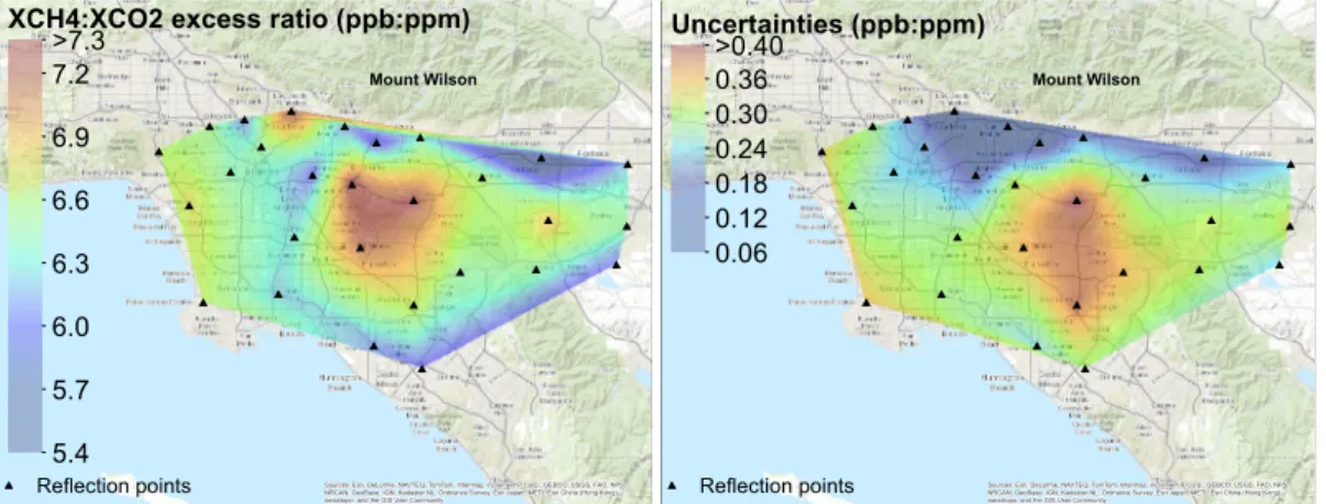
Figure 5 maps the observed XCH_4(XS)/XCO_2(XS) correlation slopes (in units

of ppb CH4(ppm CO2)− 1

) across the Los Angeles megacity using natural neigh-bor interpolation (Sibson, 1981). The mean for all 28 reflection points was 6.4±0.5 ppb CH4(ppm CO2)

−1

with individual values ranging from 5.4 to 7.3 ppb

10

CH4(ppm CO2)− 1

. Elevated XCH4(XS)/XCO2(XS) ratios were observed in west

Pasadena and in the eastern side of the Los Angeles megacity.

Spatial gradients among reflection points became weaker as distance from Mount Wilson increased. Stronger spatial gradients were observed among the closer reflec-tion points in the basin, that is, west Pasadena, Santa Anita Park and East Los Angeles,

15

while weaker spatial gradients were observed among the more distant reflection points, such as Long Beach, Marina Del Rey and North Orange County. Measurements were averaged over a much longer slant path for the more distant reflection points, com-pared to the nearby reflection points, making the measurements for the more distant reflection points less sensitive to local/point sources. Bootstrap analysis (Efron and

Tib-20

shirani, 1993) was performed to make sure that the spatial variations of the correlation slopes were not a result of sampling bias among the 28 reflection points. The uncer-tainties in the correlation slopes became larger with increasing distance from Mount Wilson due to the decreased data quality, as the measurement path in the Los Ange-les megacity became longer. (More data were filtered out for targets further from the

25

instrument, mostly because of aerosol loading.)

The CLARS-FTS observations in west Pasadena are in good agreement with TCCON measurements at the Jet Propulsion Laboratory, which showed a ratio of 7.8±0.8 ppb CH4(ppm CO2)

−1

(13)

ACPD

14, 17037–17066, 2014

California

K. W. Wong et al.

Title Page

Tables Figures

◭ ◮

Back Close

Full Screen / Esc

Discussion

P

a

per

|

Discus

sion

P

a

per

|

Discussion

P

a

per

|

Discussion

P

a

per

|

TCCON and the CLARS-FTS are to the relative change in the ratio over time, diff

er-ence measurement geometry, and/or the different approach in determining the excess

ratio. A number of in situ ground and aircraft measurements of CO2and CH4have been

performed recently with the goal of quantifying GHG emissions in the megacity. A list of

CH4: CO2ratios reported by these observations is shown in Table 4. These

observa-5

tions reported ratios ranging from 6.10 to 6.74 ppb CH4(ppm CO2)−

1

(Wennberg et al., 2012; Peischl et al., 2013; S. Newman and Y.-K. Hsu, personal communication, 2014;

Y.-K. Hsu, personal communication, 2014). Because of the di_fferent measurement

tech-niques, measurement periods and locations, CH4: CO2ratios reported by these

stud-ies are not directly comparable to column measurements. However, the CLARS-FTS

10

observations of CH₄: CO₂ratios show consistency with these measurements.

4 Discussion

4.1 Analysis assumptions

A number of assumptions are involved in deriving the CH4: CO2emission ratios. These

are described in this subsection.

15

– XCH_4(XS) and XCO_2(XS)are correlated even though the two GHGs are not

emit-ted from the same sources. CH4and CO2have chemical lifetimes that are much

longer than the timescales for mesoscale transport and therefore behave like inert

tracers in the boundary layer. Even if emitted from different sources, atmospheric

processes in the boundary layer will result in mixing on relatively short timescales

20

(typical mixing timescale in the PBL is on the order of 10–20 min, Stull, 1988). CLARS-FTS samples air masses that have undergone this short timescale

mix-ing. The high degree of correlation observed between XCH4(XS)and XCO2(XS)for

all 28 reflection points supports this mixing assumption over the entire area of the LA basin.

(14)

ACPD

14, 17037–17066, 2014

California

K. W. Wong et al.

Title Page

Tables Figures

◭ ◮

Back Close

Full Screen / Esc

Discussion

P

a

per

|

Discus

sion

P

a

per

|

Discussion

P

a

per

|

Discussion

P

a

per

|

– The slope of the XCH_4(XS): XCO_2(XS) correlation observed at each LABS

mea-surement point is sensitive to both the relative emissions over a horizontal path weighted toward the reflection point, and the composition of the air mass ad-vected into the atmospheric path. The long optical path in the boundary layer and the effect of advection smear out the effects of local emission ratio variations. This

5

smearing is different for each reflection point. Future work will deconvolve these

effects using an atmospheric transport model which will include advection,

bound-ary layer mixing, surface emissions and ray-tracing of the optical path sampled by CLARS-FTS on a 1–2 km grid.

– The effect of aerosol scattering on the XCH4(XS): XCO2(XS)slopes is assumed to

10

be negligible. Using a two-stream numerical radiative transfer model constrained by AERONET aerosol optical depths in the near-infrared, Zhang et al. (2014)

showed that the bias in the retrieved XCO2 from CLARS-FTS LABS

measure-ments does not exceed 1 %, using data that have passed the filter criteria de-scribed above. This bias is caused by the wavelength dependence of aerosol

15

scattering and absorption between the CO2absorption band at 1.61 µm, and the

O₂absorption band at 1.27 µm. Since the CO₂and CH₄observations used in this

analysis are retrieved at nearly identical wavelengths (1.61 µm vs. 1.66 µm), the

aerosol-induced bias on XCO2 and XCH4 should be nearly identical and cancel

out in the ratio. Uncertainties due to aerosol scattering on the CLARS-FTS XCO₂

20

and XCH4 observations will be reduced significantly in the next version of the

CLARS-FTS retrieval algorithm which will consider aerosol scattering explicitly in the forward model (Zhang et al., 2014).

– The number of discrete reflection points (28 plus the direct solar path) is suffi

-cient to characterize the average emission ratio over the Los Angeles megacity.

25

The CLARS-FTS LABS mode spans slant distances in the range 4–40 km in the

Los Angeles PBL, and therefore should have sufficient spatial coverage of the

(15)

ACPD

14, 17037–17066, 2014

California

K. W. Wong et al.

Title Page

Tables Figures

◭ ◮

Back Close

Full Screen / Esc

Discussion

P

a

per

|

Discus

sion

P

a

per

|

Discussion

P

a

per

|

Discussion

P

a

per

|

distribution of the reflection points with respect to coverage of emission sources, aerosol bias, albedo variability, locations of other stations in the monitoring net-work, and other parameters.

– Averaging the monthly average XCH₄/XCO₂ ratio over a two-year period to

de-rive annual average CH4emissions does not introduce a temporal sampling bias.

5

Certain times of the year are more likely to be influenced by cloud and aerosol events in Los Angeles and have correspondingly fewer measurements that pass the data quality filters. In our analysis the e_ffect of seasonal bias is assumed to

small. Since good correlation is observed between XCH4(XS): XCO2(XS)

through-out the year, the contribution of seasonal sampling bias, if any, has a negligible

10

e_ffect on the random error of the annual average XCH_4(XS): XCO_2(XS)correlation

slope.

4.2 Top-down CH4emissions from CLARS-FTS observations

With the assumptions described in the previous subsection, we estimate the top-down

annual CH₄ emission for the Los Angeles megacity based on the CLARS-FTS

obser-15

vations. The CARB reported an annual statewide CO2 emission of 387 Tg CO2year−

1

for 2011 (California Air Resources Board, http://www.arb.ca.gov/app/ghg/2000_2011/

ghg_sector.php). Since the majority of CO₂ emissions are from fossil fuel combustion,

we assumed that the CO2emissions are spatially distributed by population in the state.

We apportioned the statewide emissions by population in the Los Angeles megacity,

20

which is 43 % of statewide population, to estimate the bottom-up emission for the Los

Angeles megacity (http://www.census.gov/). The bottom-up CO2emission inventory for

the Los Angeles megacity was thus 166±23 Tg CO2year−

1

in 2011, assuming 10 %

uncertainties in both the CARB statewide CO2emission and the spatial distribution of

emissions by population. For the bottom-up CH₄emission in the Los Angeles megacity,

25

(16)

ACPD

14, 17037–17066, 2014

California

K. W. Wong et al.

Title Page

Tables Figures

◭ ◮

Back Close

Full Screen / Esc

Discussion

P

a

per

|

Discus

sion

P

a

per

|

Discussion

P

a

per

|

Discussion

P

a

per

|

apportioned by population. This gave a bottom-up CH₄ emission inventory of 0.28 Tg

CH₄year−1in the Los Angeles megacity in 2011. Using the bottom-up emission

inven-tory of CO2 for the Los Angeles megacity and the CH4: CO2 ratio observed by the

CLARS-FTS, we derived the CH4emission inventory using Eq. (3), where ECH₄|top-down

is the top-down CH₄emissions inferred by the CLARS-FTS observations, E_CO

2|bottom-up

5

is the bottom-up CO2emissions,

XCH₄

XCO₂|slopeis the XCH4(XS)/XCO2(XS)ratio observed by

the FTS and MW_MWCO2

CH4 is the ratio of molecular weight of CO2and CH4.

ECH₄|top-down=ECO₂|bottom-up×

XCH₄

XCO₂|slope×

MW_CH

4

MWCO₂

(3)

The derived CH₄emission inventory was 0.39±0.06 Tg CH₄year−1 in the Los

Ange-les megacity assuming a 10 % uncertainty in the CARB bottom-up CO2emission. The

10

derived CH4 emission inventory was 18–61 % larger than the bottom-up emission

in-ventory in 2011. This is in good agreement with recent studies (Wunch et al., 2009; Hsu et al., 2010; Wennberg et al., 2012; Peischl et al., 2013; Jeong et al., 2013).

Because of the spatial and temporal variations of CH4: CO2ratio in the Los Angeles

megacity, the derived CH₄ emission based on local observations can be biased. For

15

instance, if we were to evaluate the bottom-up CH4emission inventory by our

observa-tions in west Pasadena only, the derived CH4 emission inventory for the Los Angeles

megacity would be overestimated by 14 %, since the west Pasadena target observed a CH4: CO2slope that is 14 % larger than the average slope of the 28 reflection points. Therefore, to quantify and to reduce uncertainties in carbon emissions from the Los

20

Angeles megacity or any other urban areas which are highly heterogeneous, it is im-portant to have measurements which provide both spatial and temporal coverage. It

is challenging to quantify individual point sources of CH4. Further investigations need

to be performed to link the CLARS-FTS observations to emissions from landfills, oil extraction and natural gas pipeline leakage.

(17)

ACPD

14, 17037–17066, 2014

California

K. W. Wong et al.

Title Page

Tables Figures

◭ ◮

Back Close

Full Screen / Esc

Discussion

P

a

per

|

Discus

sion

P

a

per

|

Discussion

P

a

per

|

Discussion

P

a

per

|

4.3 Relevance to future satellite GHG observations

This study has shown that spatially resolved CH4: CO2 emission ratio measurements

can be made over a megacity domain (hundreds of km2) using a remote sensing

method that simulates the observations from an imaging spectrometer such as GEO-FTS from geostationary orbit. From GEO, the field of regard is approximately one-third

5

of the Earth below 60◦. latitude. Operating as a hosted payload from a commercial

com-munications satellite, measurements of XCO₂, XCH₄, XCO and solar-induced

chloro-phyll fluorescence (SIF) will be made every 1–2 h during daylight with a pixel footprint of 2–3 km at the sub-satellite point with retrieval precisions comparable to those obtained from CLARS-FTS (Fu et al., 2014). In the near future, a two-dimensional imaging FTS

10

similar to GEO-FTS will be deployed at CLARS to increase the spatial density of the retrievals.

5 Conclusions

This study is the first to map GHGs in the Los Angeles megacity using ground-based remote sensing technique. It combines the unique vista from Mount Wilson and

high-15

sensitivity measurements made by the CLARS-FTS to simulate satellite observations. Persistent space and time resolved observations of GHG in the Los Angeles megac-ity over a two-year period in 2011–2013 and a tracer-to-tracer correlation analysis are used to reveal interesting spatial pattern of CH4: CO2ratio in the megacity. The slope

of the correlations between XCH_4(XS) and XCO_2(XS) showed significant spatial

varia-20

tions ranging from 5.4 to 7.3 ppb CH4(ppm CO2)−

1

, with an average of 6.4±0.5 ppb

CH₄(ppm CO₂)−1, indicating that there is spatial heterogeneity in the megacity. Using

the CARB bottom-up emission inventory of CO2, we derived the CH4 emission

inven-tory of the Los Angeles megacity in 2011–2013 to be 0.39±0.06 Tg CH4year−

1

, which

was 18–61 % above the bottom-up CH4emission inventory. Good agreements among

25

(18)

ACPD

14, 17037–17066, 2014

California

K. W. Wong et al.

Title Page

Tables Figures

◭ ◮

Back Close

Full Screen / Esc

Discussion

P

a

per

|

Discus

sion

P

a

per

|

Discussion

P

a

per

|

Discussion

P

a

per

|

a robust measurement technique that can quantify and track GHG emissions in the Los

Angeles megacity in an efficient way. The CLARS-FTS also demonstrates the

poten-tial success for future satellite mission to quantify carbon emissions from megacities from space. The heterogeneity characteristics in the megacity can lead to a 14 %

un-certainty in the derived top-down CH4emissions if only observations in west Pasadena

5

are used. However, due to the complexity of the measurement geometry of the CLARS-FTS observations, it is challenging to pinpoint local sources or to derive a map of local

CH4: CO2 emission ratios at this point. Additional future work needs to be done. The

CLARS-FTS observations, which span the Los Angeles megacity continuously, fill the gap between the local measurements that provide long-term observations but are too

10

sensitive to local emissions, and aircraft data that provides intense spatial and tempo-ral observations yet are too expensive to carry out continuously throughout the year. However, it is necessary to combine the CLARS-FTS observations with in-situ ground

and aircraft data for a long-term GHG monitoring e_ffort in the megacity.

Acknowledgements. The authors thank our colleagues and D. Wunch (California Institute of

15

Technology), J. Stutz (University of California, Los Angeles) and G. Keppel-Aleks (University of Michigan) for helpful comments. Support from the California Air Resources Board, NOAA Climate Program, NIST GHG and Climate Science Program and JPL Earth Science and Tech-nology Directorate is gratefully acknowledged. Y. L. Yung, was supported in part by NASA grant NNX13AK34G to the California Institute of Technology and the KISS program of Caltech.

20

References

Aben, I., Hasekamp, O., and Hartmann, W.: Uncertainties in the space-based measurements of CO₂columns due to scattering in the Earth’s atmosphere, J. Quant. Spectrosc. Ra., 104, 450–459, 2007.

Crisp, D., Fisher, B. M., O’Dell, C., Frankenberg, C., Basilio, R., Bösch, H., Brown, L. R.,

Cas-25

(19)

ACPD

14, 17037–17066, 2014

California

K. W. Wong et al.

Title Page

Tables Figures

◭ ◮

Back Close

Full Screen / Esc

Discussion

P

a

per

|

Discus

sion

P

a

per

|

Discussion

P

a

per

|

Discussion

P

a

per

|

Suto, H., Taylor, T. E., Thompson, D. R., Wennberg, P. O., Wunch, D., and Yung, Y. L.: The ACOS CO₂ retrieval algorithm – Part II: Global XCO₂ data characterization, Atmos. Meas. Tech., 5, 687–707, doi:10.5194/amt-5-687-2012, 2012.

Efron, B. and Tibshirani, R.: An Introduction to the Bootstrap, Vol. 57, CRC press, Boca Raton, Florida, USA, 1993.

5

Fu, D., Pongetti, T. J., Blavier, J.-F. L., Crawford, T. J., Manatt, K. S., Toon, G. C., Wong, K. W., and Sander, S. P.: Near-infrared remote sensing of Los Angeles trace gas distributions from a mountaintop site, Atmos. Meas. Tech., 7, 713–729, doi:10.5194/amt-7-713-2014, 2014. Hsu, Y.-K., VanCuren, T., Park, S., Jakober, C., Herner, J., FitzGibbon, M., Blake, D. R., and

Par-rish, D. D.: Methane emissions inventory verification in southern California, Atmos. Environ.,

10

44, 1–7, 2010.

Jeong, S., Hsu, Y.-K., Andrews, A. E., Bianco, L., Vaca, P., Wilczak, J. M., and Fischer, M. L.: A multitower measurement network estimate of California’s methane emissions, J. Geophys. Res.-Atmos., 118, 11339–11351, doi:10.1002/jgrd.50854, 2013.

Key, R., Sander, S., Eldering, A., Blavier, J-F, Bekker, D., Manatt, K., Rider, D., and Wu, Y.-H.:

15

The geostationary fourier transform spectrometer, Proc. SPIE, 8515, doi:10.1117/12.930257, 2012.

Kort, E. A., Angevine, W. M., Duren, R., and Miller, C. E.: Surface observations for monitoring urban fossil fuel CO₂ emissions: Minimum site location requirements for the Los Angeles megacity, J. Geophys. Res.-Atmos., 118, 1577–1584, doi:10.1002/jgrd.50135, 2013.

20

Mandrake, L., Frankenberg, C., O’Dell, C. W., Osterman, G., Wennberg, P., and Wunch, D.: Semi-autonomous sounding selection for OCO-2, Atmos. Meas. Tech., 6, 2851–2864, doi:10.5194/amt-6-2851-2013, 2013.

Newman, S., Jeong, S., Fischer, M. L., Xu, X., Haman, C. L., Lefer, B., Alvarez, S., Rap-penglueck, B., Kort, E. A., Andrews, A. E., Peischl, J., Gurney, K. R., Miller, C. E., and

25

Yung, Y. L.: Diurnal tracking of anthropogenic CO₂ emissions in the Los Angeles basin megacity during spring 2010, Atmos. Chem. Phys., 13, 4359–4372, doi:10.5194/acp-13-4359-2013, 2013.

O’Dell, C. W., Connor, B., Bösch, H., O’Brien, D., Frankenberg, C., Castano, R., Christi, M., Eldering, D., Fisher, B., Gunson, M., McDuffie, J., Miller, C. E., Natraj, V., Oyafuso, F.,

Polon-30

(20)

ACPD

14, 17037–17066, 2014

California

K. W. Wong et al.

Title Page

Tables Figures

◭ ◮

Back Close

Full Screen / Esc

Discussion

P

a

per

|

Discus

sion

P

a

per

|

Discussion

P

a

per

|

Discussion

P

a

per

|

Peischl, J., Ryerson, T. B., Brioude, J., Aikin, K. C., Andrews, A. E., Atlas, E., Blake, D., Daube, B. C., de Gouw, J. A., Dlugokencky, E., Frost, G. J., Gentner, D. R., Gilman, J. B., Goldstein, A. H., Harley, R. A., Holloway, J. S., Kofler, J., Kuster, W. C., Lang, P. M., Nov-elli, P. C., Santoni, G. W., Trainer, M., Wofsy, S. C., and Parrish, D. D.: Quantifying sources of methane using light alkanes in the Los Angeles basin, California, J. Geophys. Res.-Atmos.,

5

118, 4974–4990, doi:10.1002/jgrd.50413, 2013.

Sibson, R.: A brief description of natural neighbor interpolation, in: Interpreting Multivariate Data, edited by: Barnet, V., Wiley, Chichester, 21–36, 1981.

Spurr, R. J: VLIDORT: A linearized pseudo-spherical vector discrete ordinate radiative transfer code for forward model and retrieval studies in multilayer multiple scattering media, J. Quant.

10

Spectrosc. RA., 102, 2, 316–342, 2006.

Stull, R: An Introduction to Boundary Layer Meteorology, Springer, the Netherlands, 1988. Washenfelder, R. A. and Wennberg, P. O.: Troposheric methane retrieved from

ground-based near-IR solar absorption spectra, Geophys. Res. Lett., 30, 23, 2226, doi:10.1029/2003GL017969, 2003.

15

Washenfelder, R. A., Toon, G. C., Blavier, J.-F., Yang, Z., Allen, N. T., Wennberg, P. O., Vay, S. A., Matross, D. M., and Daube, B. C.: Carbon dioxide column abundances at the Wisconsin Tall Tower site, J. Geophys. Res., 111, D22305, doi:10.1029/2006JD007154, 2006.

Wennberg, P. O., Mui, W., Wunch, D., Kort, E. A., Blake, D. R. Atlas, E. L., Santoni, G. W., Wofsy, S. C., Diskin, G. S., Joeng, S., and Fischer, M. L.: On the sources of methane to the

20

Los Angeles atmosphere, Environ. Sci. Technol., 46, 9282–9289, doi:10.1021/es301138y, 2012.

Wunch, D., Wennberg, P. O.,Toon, G. C., Keppel-Aleks, G., and Yavin, Y. G.: Emissions of greenhouse gases from a North American megacity, Geophys. Res. Lett., 36, L15810, doi:10.1029/2009GL039825, 2009.

25

Wunch, D., Toon, G. C., Blavier, J. L., Washenfelder, R. A., Notholt, J., Connor, B. J., Grif-fith, D. W., Sherlock, V., and Wennberg, P. O.: The total carbon column observing network, Philos. T. Roy. Soc. A, 369, 2087–2112, 2011.

Yoshida, Y., Ota, Y., Eguchi, N., Kikuchi, N., Nobuta, K., Tran, H., Morino, I., and Yokota, T.: Retrieval algorithm for CO₂ and CH₄ column abundances from short-wavelength infrared

30

(21)

ACPD

14, 17037–17066, 2014

California

K. W. Wong et al.

Title Page

Tables Figures

◭ ◮

Back Close

Full Screen / Esc

Discussion

P

a

per

|

Discus

sion

P

a

per

|

Discussion

P

a

per

|

Discussion

P

a

per

|

Zhang, Q., Natraj, V., Li, K., Shia, R., Fu, D., Pongetti, T., Sander, S. P., and Yung, Y. L.: Influence of aerosol scattering on the retrieval of CO₂mixing ratios: a case study using measurements from the California Laboratory for Atmospheric Remote Sensing (CLARS), Geophys. Res. Lett., in preparation, 2014.

California Air Resources Board: Greenhouse gas emission inventory – Query tool for years

5

(22)

ACPD

14, 17037–17066, 2014

California

K. W. Wong et al.

Title Page

Tables Figures

◭ ◮

Back Close

Full Screen / Esc

Discussion

P

a

per

|

Discus

sion

P

a

per

|

Discussion

P

a

per

|

Discussion

P

a

per

|

Table 1.List of the 29 reflection points on Mount Wilson and in the Los Angeles megacity.

Target Latitude Longitude Slant *Slant path Footprint

distance in PBL (km) (km2) from FTS (km)

1 Spectralon®, Mount Wilson 34.22 −118.06 0.01 0 0

2 Santa Anita Park 34.14 −118.04 9.2 4.2 0.04

3 west Pasadena 34.17 −118.17 11.5 5.9 0.09

4 Santa Fe Dam 34.11 −117.97 14.9 6.8 0.17

5 East Los Angeles 34.05 −118.12 20.2 9.2 0.41

6 Fwy 210 34.12 −117.87 20.9 10.1 0.49

7 Downtown (near) 34.10 −118.23 21.1 9.6 0.47

8 Glendale 34.15 −118.27 21.4 10.0 0.50

9 Fwys 60 and 605 34.03 −118.03 21.7 9.5 0.49

10 Universal City 34.14 −118.35 28.8 13.4 1.23

11 Fwy 60, City of Industry 34.00 −117.88 29.6 13.7 1.33

12 Downtown (far) 34.05 −118.31 29.7 12.9 1.25

13 Downey 33.93 −118.16 33.9 14.5 1.84

14 La Mirada 33.91 −118.01 35.2 15.3 2.09

15 Pomona 34.04 −117.73 36.7 18.1 2.70

16 Santa Monica Mountains 34.09 −118.47 40.9 20.2 3.74

17 Marina Del Rey 33.99 −118.40 41.0 17.3 3.22

18 Rancho Cucamonga 34.08 −117.59 46.1 24.0 5.66

19 Long Beach 33.82 −118.20 46.5 19.6 4.70

20 North Orange County 33.86 −117.78 47.8 21.3 5.38

21 Angels Stadium 33.80 −117.88 49.8 21.5 5.89

22 Norco 33.96 −117.57 53.5 25.3 8.01

23 Palos Verdes 33.81 −118.37 54.2 23.7 7.70

24 Huntington Beach 33.72 −117.98 56.2 23.8 8.32

25 Corona 33.87 −117.60 56.0 28.8 10.71

26 Orange Country Airport 33.68 −117.86 63.3 26.7 11.86

27 Fontana 34.07 −117.39 64.3 33.8 15.46

28 Riverside 33.95 −117.39 68.5 34.1 17.75

29 Lake Mathews 33.88 −117.42 70.7 39.1 21.62

∗_{Slant paths in PBL are estimated assuming a uniform PBL height of 700 m, which was the average PBL height observed}

(23)

ACPD

14, 17037–17066, 2014

California

K. W. Wong et al.

Title Page

Tables Figures

◭ ◮

Back Close

Full Screen / Esc

Discussion

P

a

per

|

Discus

sion

P

a

per

|

Discussion

P

a

per

|

Discussion

P

a

per

|

Table 2.Data filter criteria.

Filter Criteria

High clouds SVO O_{2 SCD_retrieved}: O_{2 SCD_Geometric}>1.1 or<1

Low clouds and/or aerosol LABS O_{2 SCD_retrieved}: O_{2 SCD_geometric}>1.1 or<0.9

Large SZA SZA>₇₀◦

Low SNR SNR<₁₀₀

Poor spectral fitting Fitting residual RMS>_{1 standard deviation above}

(24)

ACPD

14, 17037–17066, 2014

California

K. W. Wong et al.

Title Page

Tables Figures

◭ ◮

Back Close

Full Screen / Esc

Discussion

P

a

per

|

Discus

sion

P

a

per

|

Discussion

P

a

per

|

Discussion

P

a

per

|

Table 3.List of correlation slopes of XCH_4(XS): XCO_2(XS)and their uncertainties (one standard deviation) observed by the CLARS-FTS between the period of September 2011 and October 2013.

Target XCH_4(xs)/XCO_2(xs) Uncertainties

(ppb/ppm) (ppb/ppm)

Santa Anita Park 6.09 0.05

west Pasadena 7.28 0.09

Santa Fe Dam 5.85 0.12

East Los Angeles 5.99 0.15

Fwy 210 6.26 0.20

Downtown (near) 6.42 0.21

Glendale 6.04 0.20

Fwys 60 and 605 7.34 0.31

Universal City 6.47 0.28

Fwy 60, City of Industry 7.25 0.41

Downtown (far) 6.33 0.23

Downey 6.24 0.29

La Mirada 7.13 0.35

Pomona 6.52 0.25

Santa Monica Mountains 6.55 0.33

Marina Del Rey 6.75 0.27

Rancho Cucamonga 5.35 0.15

Long Beach 6.18 0.28

North OC 6.41 0.35

Angels Stadium 6.65 0.39

Norco 6.87 0.31

Palos Verdes 6.59 0.34

Huntington Beach 6.10 0.24

Corona 6.40 0.30

Orange Country Airport 5.99 0.29

Fontana 6.18 0.23

Riverside 6.40 0.32

(25)

ACPD

14, 17037–17066, 2014

California

K. W. Wong et al.

Title Page

Tables Figures

◭ ◮

Back Close

Full Screen / Esc

Discussion

P

a

per

|

Discus

sion

P

a

per

|

Discussion

P

a

per

|

Discussion

P

a

per

|

Table 4.Comparisons of CH₄: CO₂ ratios and derived top-down CH₄ emissions among vari-ous measurements in the Los Angeles megacity. Please note that it is difficult to compare the uncertainties due to the different measurement techniques.

Measurement (Location, period)

CH4: CO2ratio

(ppb:ppm)

Derived top-down CH4emission

(Tg CH4year

−1

)

Measurement type References

TCCON

(Pasadena, Aug 2007–Jun 2008)

7.80±0.80 0.40±0.10 0.60±0.10

Column (FTS) Wunch et al. (2009)

ARCTAS (LA, Jun 2008)

6.74±0.58 0.47±0.10 Aircraft in-situ (Picarro)

Wennberg et al. (2012)

CalNex

(LA, May 2010–Jun 2010)

6.70±0.01 0.41±0.04 Aircraft in-situ (Picarro)

Peischl et al. (2013)

Caltech

(Pasadena, Feb 2012–Aug 2012)

6.30±0.01 0.38±0.05 Surface in-situ This study

Mount Wilson

(Pasadena, Sep 2011–Jun 2013)

6.10±0.10 0.37±0.05 Surface in-situ (Picarro)

This study

CLARS-FTS, Mount Wilson (LA, Sep 2011–Oct 2013)

(26)

ACPD

14, 17037–17066, 2014

California

K. W. Wong et al.

Title Page

Tables Figures

◭ ◮

Back Close

Full Screen / Esc

Discussion

P

a

per

|

Discus

sion

P

a

per

|

Discussion

P

a

per

|

Discussion

P

a

per

|

1

2

3

(27)

ACPD

14, 17037–17066, 2014

California

K. W. Wong et al.

Title Page

Tables Figures

◭ ◮

Back Close

Full Screen / Esc

Discussion

P

a

per

|

Discus

sion

P

a

per

|

Discussion

P

a

per

|

Discussion

P

a

per

|

1

2

100

80

60

40

20

0 D

a

ta

p

a

ss

t

h

rou

g

h

ﬁ

lt

e

rs

(

%

)

80

60

40

20

0 Slant distance in the basin (km)

(28)

ACPD

14, 17037–17066, 2014

California

K. W. Wong et al.

Title Page

Tables Figures

◭ ◮

Back Close

Full Screen / Esc

Discussion

P

a

per

|

Discus

sion

P

a

per

|

Discussion

P

a

per

|

Discussion

P

a

per

|

1

2

3

4

Figure 3.Upper panel shows the raw data and bottom panel shows the filtered data. Diurnal variations of SVO (grey) and LABS, west Pasadena (red) and Santa Anita Park (blue), XCO₂ and XCH₄from around 08:30 to 16:30 local time (PST) on seven consecutive days in May 2012. Error bars represent the RMS of the retrieval spectral fitting residual. Bad data points, such as data taken in the cloudy morning of 11 May, were removed from the filtered data set. From 5–9 May, the FTS was operated in the target mode, taking alternate measurements among SVO, west Pasadena and Santa Anita Park. On 10–11 May, standard measurement cycle was performed, resulting in fewer measurements from each target.

(29)

ACPD

14, 17037–17066, 2014

California

K. W. Wong et al.

Title Page

Tables Figures

◭ ◮

Back Close

Full Screen / Esc

Discussion

P

a

per

|

Discus

sion

P

a

per

|

Discussion

P

a

per

|

Discussion

P

a

per

|

1

2 Figure 4.Correlations between XCH4(XS) (ppb) and XCO2(XS) (ppm) for west Pasadena and

Santa Anita Park between the period of September 2011 and October 2013.

(30)

ACPD

14, 17037–17066, 2014

California

K. W. Wong et al.

Title Page Abstract Introduction Conclusions References Tables Figures ◭ ◮ ◭ ◮ Back Close

Full Screen / Esc

Printer-friendly Version Interactive Discussion Discussion P a per | Discus sion P a per | Discussion P a per | Discussion P a per | # # # # # # # # # # # # # # # # # # # # # # # # # # # # Mount Wilson

Sources: Esri, DeLorme, NAVTEQ, TomTom, Intermap, increment P Corp., GEBCO, USGS, FAO, NPS, NRCAN, GeoBase, IGN, Kadaster NL, Ordnance Survey, Esri Japan, METI, Esri China (Hong Kong), swisstopo, and the GIS User Community

# Reflection points

XCH4:XCO2 excess ratio (ppb:ppm) >7.3 7.2 6.9 6.6 6.3 6.0 5.7 5.4 # # # # # # # # # # # # # # # # # # # # # # # # # # # # Mount Wilson

Sources: Esri, DeLorme, NAVTEQ, TomTom, Intermap, increment P Corp., GEBCO, USGS, FAO, NPS, NRCAN, GeoBase, IGN, Kadaster NL, Ordnance Survey, Esri Japan, METI, Esri China (Hong Kong), swisstopo, and the GIS User Community

# Reflection points

Uncertainties (ppb:ppm) >0.40 0.36 0.30 0.24 0.18 0.12 0.06