www.ocean-sci.net/10/633/2014/ doi:10.5194/os-10-633-2014
© Author(s) 2014. CC Attribution 3.0 License.
The surface thermal signature and air–sea coupling over the
Agulhas rings propagating in the South Atlantic Ocean interior
J. M. A. C. Souza1,*, B. Chapron1, and E. Autret1
1Laboratoire d’Oceanographie Spatiale (LOS), IFREMER, Centre Brest, 29280, Plouzané, France
*now at: Department of Oceanography, School of Ocean and Earth Science Technology (SOEST), University of Hawaii, 1000 Pope Rd., MSB, Honolulu, 96822 HI, USA
Correspondence to:J. M. A. C. Souza ([email protected])
Received: 9 October 2013 – Published in Ocean Sci. Discuss.: 5 December 2013 Revised: 14 May 2014 – Accepted: 30 May 2014 – Published: 9 July 2014
Abstract.The surface signature of Agulhas rings propagat-ing across the South Atlantic Ocean is observed based on three independent data sets: Advanced Microwave Scanning Radiometer for the Earth Observing System/Tropical Rain-fall Measuring Mission (TRMM) Microwave Imager (TMI) (TMI/AMSR-E) satellite sea surface temperature, Argo pro-filing floats and a merged winds product derived from scat-terometer observations and reanalysis results. A persistent pattern of cold (negative) sea surface temperature (SST) anomalies in the eddy core, with warm (positive) anomalies at the boundary, is revealed. This pattern contrasts with the classical idea of a warm core anticyclone. Taking advantage of a moving reference frame corresponding to the altimetry-detected Agulhas rings, modifications of the surface winds by the ocean-induced currents and SST gradients are evalu-ated using satellite SST and wind observations. As obtained, the averaged stationary thermal expression and mean eddy-induced circulation are coupled to the marine atmospheric boundary layer, leading to surface wind anomalies. Conse-quently, an average Ekman pumping associated with these mean surface wind variations consistently emerges. This av-erage Ekman pumping is found to explain very well the SST anomaly signatures of the detected Agulhas rings. Particu-larly, this mechanism seems to be the key factor determining that these anticyclonic eddies exhibit stationary imprints of cold SST anomalies near their core centers. A residual phase with the maximum sea surface height (SSH) anomaly and wind speed anomaly is found to the right of the mean wind direction, apparently maintaining a coherent stationary ther-mal expression coupled to the marine atmospheric boundary layer.
1 Introduction
The Agulhas rings are important features of the South At-lantic circulation, with particular relevance for the great ocean conveyor belt. It is believed that virtually all the up-per layer overturning circulation in the Atlantic originates from Indian Ocean leakage through Agulhas rings. Although previous studies have estimated the Agulhas rings general characteristics and pathways in the South Atlantic (e.g., Dencausse et al., 2010; Souza et al., 2011a), these do not usually include their thermal signature on the surface. More-over, studies that have observed the Agulhas rings at sea (e.g., van Aken et al., 2003) are usually restricted to newly formed eddies and do not represent their modifications along their lifetimes. The eddy surface thermal signatures and their evo-lution over time have important consequences on the air–sea fluxes, impacting the overlying marine atmospheric bound-ary layer (MABL) with possible consequences on the re-gional atmospheric circulation.
the sea front. Statistically, observed SST-induced perturba-tions on the surface wind stress or the scatterometer wind curl and divergence fields have been found to be linearly well cor-related with small scale perturbations in the crosswind and downwind SST gradients, respectively (e.g., Chelton et al., 2001, 2007; O’Neill et al., 2005, 2010). Moreover, impor-tant consequences on cloud fraction and water content of the MABL, and a reduction in rainfall have been observed for cyclones in the Southern Ocean by Frenger et al. (2013).
Considering these ocean–atmosphere interactions, Businger and Shaw (1984, see the schematic diagram in their Fig. 10) earlier sketched several interactions of eddy SST imprints with the atmospheric boundary layer, and numerous studies have clearly evidenced air–sea couplings over oceanic mesoscale coherent structures (e.g., Chelton et al., 2001, 2007; Small et al., 2008). As summarized in Small et al. (2008), the main coupling mechanisms are related to (i) changes in the near-surface stability and surface stress, (ii) vertical transfer of momentum from higher atmospheric levels to the surface due to an increase of the turbulence in the boundary layer, (iii) secondary circulations associated with perturbations in the surface atmospheric pressure over the SST fronts and (iv) the impact of the oceanic eddy currents on the net momentum transferred between the atmosphere and the ocean.
The objective of this study is to characterize the surface thermal signature of Agulhas rings propagating across the South Atlantic Ocean and the associated wind perturbation. An air–sea coupling mechanism over the oceanic mesoscale eddies emerges from the relationship observed between the wind and SST patterns.
To analyze the air–sea coupling over Agulhas rings, the present work takes advantage of a moving reference frame (Lagrangian) corresponding to altimetry-detected mesoscale Agulhas rings propagating in the South Atlantic basin. This approach permits the evaluation of the eddy-tracked aver-age modifications to surface winds by the sea surface tem-perature (SST) gradients, using satellite SST and wind ob-servations. Agulhas rings are the largest mesoscale eddies in the world, with large radii (165±69 km) and durations (497±233 days) (see Souza et al., 2011a). Accordingly, the Lagrangian approach can easily be implemented to reveal the persistent structures of SSH, SST and wind anomalies using standard medium-resolution satellite products, as presented in Sects. 2 and 3. Our study follows earlier investigations on the modification of the surface winds over Gulf Stream rings (Park et al., 2006), but benefit from the higher temporal sampling of surface wind and SST information over isolated altimetry-detected rings.
Three independent data sets – TMI/AMSR-E SST satellite observations, Argo profiling floats and a merged wind prod-uct derived from scatterometer measurements and a reanaly-sis – are used to describe the imprint of Agulhas rings on the SST field in Sect. 4. The evidence of the mean air–sea cou-pling over the detected rings is presented in Sect. 5, clearly
exhibiting the mean eddy/wind interactions. Maintaining the expectation that stationary thermal expression and relative air–water velocity are well expressed in the near-surface ma-rine atmospheric boundary layer, the corresponding aver-age Ekman pumping associated with the mean surface wind variations can then be evaluated. As revealed, the persistent eddy-induced Ekman pumping compares very well with the observed SST anomalies, as discussed in Sect. 6. Conclu-sions derived from the present analysis follow in Sect. 7.
2 Data
For our purposes, wind information from a blend of Quick Scatterometer (QuikSCAT) observations and reanalysis re-sults, gridded SSH from Archiving, Validation and Inter-pretation of Satellite Oceanographic (AVISO) data, blended TMI/AMSR-E SST over a four-year period (between Jan-uary 2005 and December 2008) and Argo float temperature profiles are used.
2.1 Blended wind fields
The blended wind product used in the present study is avail-able for download in NetDCF format at (ftp://ftp.ifremer. fr/ifremer/cersat/products/gridded/psi-concentration/), and a complete description is provided by Bentamy et al. (2007). To enhance the spatial and temporal resolutions (0.25◦ at synoptic times 00:00, 06:00, 12:00 and 18:00 UTC), a method has been implemented to blend the remotely sensed wind observations derived by the satellite QuikSCAT scat-terometer and by three Special Sensor Microwave Imagers (SSM/I) on board Defense Meteorological Satellite Program (DMSP) satellites F13, F14 and F15 with the European Cen-tre for Medium-Range Weather Forecasts (ECMWF) analy-ses. This provides a uninterrupted, high-resolution (∼25 km) data set of wind velocities over the eddy tracks during the an-alyzed period.
2.2 AVISO SSH data
2.3 TMI/AMSR-E SST fields
An optimally interpolated SST (OI-SST) product, combining TRMM Microwave Imager (TMI) and Advanced Microwave Scanning Radiometer for EOS (AMSR-E) data sets, is used to provide the SST over the Agulhas rings. This product provides daily “cloud free” SST maps, with approximately 25 km spatial resolution – compatible with the wind data set. The data can be downloaded and details about the optimal in-terpolation procedural can be found at www.remss.com. This data set is produced by Remote Sensing Systems and is spon-sored by the National Oceanographic Partnership Program (NOPP), the NASA Earth Science Physical Oceanography Program and the NASA Measures Discover Project.
2.4 Argo profiling floats
Argo is a global ocean observing system for the 21st century (www.argo.net) composed of approximately 3000 profiling floats, used to create 3◦×3◦×10-day resolution array be-tween 60◦S to 60◦N. These autonomous floats measure tem-perature and salinity down to 2000 m depth, every 10 days. A complete description of the Argo program and access to the data can be obtained at http://www.ARGOucsd.edu/. In the present study, we take advantage of the Argo profiles co-located with the Agulhas rings in space and time, and a de-rived mean vertical temperature anomaly structure, dede-rived by Souza et al. (2011b).
3 Methods
The present work takes advantage of a Lagrangian point of view along the eddy tracks to quantify the anomalies in the surface variables (SSH, SST and wind) over the large mesoscale Agulhas rings propagating in the South Atlantic basin.
3.1 Eddy identification and tracking algorithm
An automated method based on the SLA (Chaigneau et al., 2009) was used to identify and track the Agulhas rings. The eddy identification process is performed at each time step, or SLA map, through two stages: (1) the identification of lo-cal SLA modulus maxima corresponding to the eddy cen-ters and (2) the selection of closed SLA contours associ-ated with each eddy center. The outermost contour embed-ding only one center is considered as the eddy edge. This method is similar to the one applied by Chelton et al. (2011), and showed improved results and performance in terms of processing time when compared to other classical methods (Souza et al., 2011a).
A total of 16 Agulhas rings with durations larger than six months were identified. The results from the tracking algorithm together with the general ring characteristics are discussed by Souza et al. (2011a). A good agreement with
previous work was achieved, with “typical” Agulhas rings shed every 2–3 months and with a diameter of 150–200 km (van Sebille et al., 2010; van Aken et al., 2003). It is impor-tant to emphasize that due to the “noisy” SSH in the Agulhas Current retroflexion region, the automated method does not identify the structures in the exact moment of their formation. Therefore, the derived SST and wind anomaly signatures cor-respond to Agulhas rings propagating in the South Atlantic interior after leaving their formation region. This is important since the SST signature of newly formed Agulhas rings is in fact warm (e.g., Gladyshev et al., 2008; Arhan et al., 2011). However, when the structures propagate northwestward into the warmer South Atlantic basin their SST anomalies in re-lation to the surrounding waters become cold, as revealed in the next section.
3.2 Data cropping and spatial high-pass filtering The SST anomaly (T′)and SST-driven wind speed
variabil-ity, or wind anomaly (V′), were isolated by removing the large spatial scale variability using a “loess” smoothing func-tion with half-power filter cutoffs of 5◦latitude by 5◦ longi-tude. The cutoff wavelengths were chosen to better isolate the influence of the mesoscale eddies from the mean field and larger-scale processes, such as propagating Rossby waves. After the eddy identification and tracking processes, the ring positions are linearly interpolated from the 7-day SLA de-rived axis to daily positions compatible with the SST and wind data sets. For the comparison between wind and SST, these data sets were linearly interpolated to a 25 km resolu-tion grid in a region of 700 km (north–south and west–east) centered over the eddy core position at each time are deter-mined from the altimetry. The properties were then projected on a horizontal grid normalized by the eddy diameter at each time step. That way, the obtained spatial patterns are isolated from the variability of the eddy diameters between distinct structures and over time.
The mean wind direction over each ring at each moment was calculated and used as a reference. For the comparison between the wind and SST, all data fields were rotated to have the x axis oriented to the mean wind at each time. Cross-wind and downCross-wind SST gradients ((∂T /∂c)′and(∂T /∂d)′, respectively) and the wind divergence and vorticity ((∇.u)′ and(∇ ×u)′, respectively) were calculated at each grid point following the method described by O’Neill et al. (2010).
Figure 1.Time series of the maximum (warm) and minimum (cold)T′inside the eddy (thin lines) and absolute SST at the eddy center (thick line) for an Agulhas ring tracked between January 2005 and February 2007.
in the southern tip of the African continent (e.g., Arhan et al., 2011; Schmid et al., 2003; Garzoli et al., 1999). As an example, Arhan et al. (2011) and Gladyshev et al. (2008) ob-served anticyclonic eddies with core temperatures between 11.8◦C and 12.5◦C approximately at 43–40◦S embedded in climatological SSTs lower than 10◦C.
But when these rings leave their formation region and move to lower latitude warmer waters, the positive signature on theT′becomes less clear. Moreover, although the waters present in the eddy cores are trapped and relatively laterally isolated from the surrounding ocean (Souza et al., 2011b), fluxes in the air–sea interface and the base of the mixed layer are expected to act modifying the upper layer temperature.
Taking as an example an Agulhas ring tracked between December 2004 and February 2007, it is possible to observe in Fig. 1 that while the absolute SST at the eddy center (deter-mined from the SLA) present a seasonal cycle with a warm trend as the ring propagates northwestward, cold and warm signatures inT′are present inside the eddy and decrease to-gether over time without a clear seasonal influence. This is similar to the behavior observed for the SLA at the eddy core by Souza et al. (2011a). While these authors obtained a de-crease rate of 9.33×10⁻⁵m day−1for the SLA, a linear fit to the T′ modulus results in an amplitude decrease rate of 3.1×10⁻⁴◦C day−1. Observing the anomaly curves in Fig. 1, one can see that this decrease is, in fact, faster in the early days of the eddy lifetime and becomes smoother after the first year. The absolute values forT′are typically lower than
0.5◦C after the first year of the eddy formation. This makes it difficult to track the eddy signature in SST satellite images, especially when it approaches the warm waters of the Brazil Current.
The T′ present similar magnitude cold and warm values inside the ring core that stay in phase during the eddy life-time. However, in contrast to the warm core observed near the formation region by Arhan et al. (2011), the Hovmoller diagram of Fig. 2 reveals a persistent cold (negative) T′ at
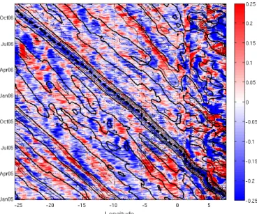
Figure 2.Hovmoller diagram of the SLA and SST anomaly (T′) along the trajectory of an Agulhas ring first observed on 24 Jan-uary 2005. The colors correspond to the SST anomalies, while the black contours present the SLA with 0.1 m interval. The thick black lines are the zero SLA contours, while the thick black dashed line present the trajectory of the eddy center. It is possible to observe that the eddy core is generally associated with cold (negative) SST anomalies.
the eddy center identified from the altimetry, and warm (pos-itive) anomalies near the eddy boundaries.
rings, indicate that all observed eddies presented persistent cold cores.
Such pattern of cold T′ in the eddy core is also present
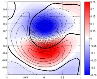
in the mean Agulhas ring vertical structure calculated from the Argo float temperature profiles by Souza et al. (2011b) (Fig. 4) for the same 16 rings analyzed in the present work. Focusing on the top layer of the water column, the mean Argo temperature anomaly section shows an eddy core dominated by cold (negative)T′while the warm (positive)T′is shifted to the left (west) of the center. The warm anomaly occupies the eddy core with depth due to the tilt between the temper-ature and velocity anomaly vertical structures. Although the mean vertical structure obtained from the Argo floats is the product of a series of simplifications used to combine profiles from different stages of the eddy lives, and it is restricted to a zonal section, it agrees with the mean spatial pattern of the eddy surface thermal signature as obtained from the TMI/AMSR-E SST product (Fig. 5). This mean surface sig-nature also shows a coldT′core with warm anomalies in the boundary, especially on the southern portion of the eddy. Al-though a large standard deviation (sd) is observed forT′this mean picture is robust, especially in the eddy core as shown by the ratio between the eddy averaged mean and sd ofT′ (see the Supplement). A similar distribution in the blended winds shows weaker (negative)V′ close to the eddy center and stronger (positive)V′at the eddy boundary. Such a rela-tionship betweenV′andT′has being previously observed by
several authors (a review is provided by Small et al., 2008). Thus, the obtained distribution ofV′reinforces the observed spatial pattern in T′. Moreover, it suggests that a coupling mechanism between the upper ocean and the MABL is re-sponsible for sustaining the observed structures.
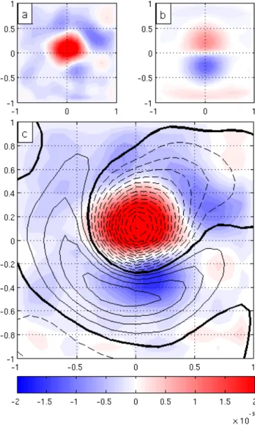
5 Evidence of air–sea coupling over the Agulhas rings As averaged, the mean spatial patterns ofV′andT′, Fig. 5,
exhibit a correlation of 0.61 with an apparent phase shift. Simply shifting the wind field position in relation to the SST and recalculating the resulting correlations, a maximum value of 0.87 is obtained for a spatial shift on the order of one quarter of the ring radius (∼50 km) to the right of the mean wind direction (downward). Since the Agulhas rings propagation region is dominated by the westerly winds, this is the same to say the wind is shifted equatorward (approx-imately 0.5◦) to the T′ center. A spatial shift between the
wind and the SST was already reported in previous studies. Considering four distinct regions (Kuroshio Current, Gulf Stream, Brazil–Malvinas confluence zone and the Agulhas Return Current), O’Neill et al. (2010) estimated a mean shift of 1◦(∼110 km). In our case, two processes contribute to the air–sea coupling over the rings: (a) the wind accelerates (de-celerates), with slight changes in wind direction, over warm (cold) SST anomalies and (b) the impact of the oceanic eddy velocities on the relative air–water velocity on diametrically
opposite sides of the eddies systematically act to modify the wind field.
Indeed, the spatial pattern for the wind perturbations in Fig. 5 suggests an influence of the oceanic eddy velocities, reducing (augmenting) the wind in the upper (lower) part of the ring. It is important here to remember that the influence of the ocean currents was removed from the scatterometer winds prior to the analysis.
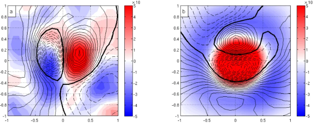
Accordingly, a coincidence in the spatial patterns of(∇.u)′ and(∂T /∂d)′is expected and observed, Fig. 6a. Taking into account the same spatial shift observed betweenV′ andT′,
the correlation changes from 0.29 to 0.83. For the relation-ship between (∇ ×u)′ and (∂T /∂c)′ (Fig. 6b), a shift of 25 km (1 grid cell) enhances the anti-correlation from−0.39 to−0.67. However, the present results are statistically robust and favor the dominant effect of the eddy-induced circulation to explain both the weaker correlation between(∇ ×u)′and (∂T /∂c)′, and the very large linear regression coefficient be-tween(∂T /∂d)′and shifted(∇.u)′, as discussed in the next section.
5.1 Linear relationship between the wind and the SST Linear relationship between the wind stress curl and diver-gence, and the crosswind and downwind SST gradients were originally observed by Chelton et al. (2001) over energetic regions of the world ocean, where strong and persistent SST fronts are present. However, it is still not clear if the same relationships hold for the less energetic ocean interior, with the sporadic occurrence of eddies. This is the case of the Agulhas rings that propagate across the South Atlantic inte-rior. Following this idea, linear fits between the binned prop-erties were obtained and their respective slopes calculated. To investigate the relationship between the wind and SST, the wind propertiesV′,(∇ ×u)′and(∇.u)′were binned in
function ofT′,(∂T /∂c)′and(∂T /∂d)′, respectively. All the data including the complete time span of all 16 identified Ag-ulhas rings were used, without spatial shift correction.
The linear relationship betweenT′andV′in Fig. 7 shows a similar slope (0.31) as the relationship observed for the Gulf Stream region (0.27) by O’Neill et al. (2010). TheT′ values are concentrated in the range±1◦C, corresponding to perturbations inV′of ±0.6 m s−1. These values are smaller than observed by previous authors, reflecting the fact these rings represent a weaker perturbation in the SST field when compared to western boundary current frontal systems. But the comparable values of the slopes indicate a similar cou-pling between the SST and the wind speed over the struc-tures, suggesting the same mechanisms are dominant.
Figure 3.Time series of the meanT′in the eddy thermal centers (thick line) showing the persistence of negative (cold) values. The thin gray lines indicate the maximum and minimum values ofT′at the eddy thermal centers between the different rings identified at each time, showing that all observed structures presented cold cores.
Figure 4.Top 100 m of the Agulhas rings meanT′vertical structure (c.i. 0.1◦C) obtained from the Argo float vertical profiles by Souza et al. (2011b) (c.i.: contour interval). The red contours indicate the 0◦CT′, while the thick black lines delimit the water trapped region following the criteria by Flierl (1981). The cold (negative)T′ dom-inates the eddy core near the surface, while the warm (positive)T′ is shifted to the left (west).
and the SST gradients over the Agulhas rings. In particular, the case of the(∇.u)′×(∂T /∂d)′shows a high slope, which means the wind convergence presents a strong response to the SST structure. The observed differences in the linear fit slope indicate that characteristics other than the SST may be influencing the MABL winds. Aspects such as the mean at-mospheric circulation and latitude impact the air–sea cou-pling and are analyzed in the next section.
5.2 Mean characteristics influencing the coupling Several physical mechanisms influence the air–sea coupling over oceanic mesoscale structures. Small et al. (2008) pro-pose as main processes the modification of the near-surface stability, the mixing of momentum, heat and humidity from higher levels into the MABL due to the increased turbu-lence, the formation of secondary circulation cells related to
Figure 5. Map of the mean perturbation wind speed (V′ color contours) and T′ (black contours – c.i. 0.01◦C) obtained from the 16 Agulhas rings observed between January 2005 and Decem-ber 2008. The thick black line represents the 0◦CT′, the continuous lines positive values and the dashed lines negative values ofT′. The figures’ axes represent the distances from the eddy centers normal-ized by the eddy diameters.
perturbations in the pressure field and the impact of oceanic eddy velocities on the surface shear. Diverse environmental properties influence these mechanisms, altering their relative balance over the eddies.
Using the differences between the environmental con-ditions influencing the 16 Agulhas rings identified in the present study it is possible to investigate the importance of the environmental properties on the coupling. To achieve this, the correlations and slopes betweenV′×T′,(∇.u)′×
Figure 6. (a)(∇.u)′ as color contours and(∂T /∂d)′as black contours – c.i. 1×10⁻⁷◦C per 100 km.(b)(∇ ×u)′(color contours) and (∂T /∂c)′(black contours – c.i. 1×10⁻⁷◦C per 100 km). The thick black lines represent the 0◦C per 100 km contours, the continuous lines positive values and the dashed lines negative values ofT′gradient. The figures’ axes represent the distances from the eddy centers normalized by the eddy diameters.
Table 1.Correlations between the slopes and correlation factors that indicate the air–sea coupling over the 16 Agulhas rings observed in the present study. The emphasized values correspond to the correlations statistically relevant to the 95 % level.
Slope Correlation
T′×V′ −(∇ ×u)′×(∂T /∂c)′ (∇.u)′×(∂T /∂d)′ T′×V′ −(∇ ×u)′×(∂T /∂c)′ (∇.u)′×(∂T /∂d)′ ¯
V 60% 74% 25 % 35 % 45% 50%
Mean Latitude –70% –56% −11 % –52% –51% –57%
Mean Diameter −19 % −22 % −15 % −2 % −4 % −7 %
Mean Amplitude 11 % −14 % −3 % 11 % −21 % 12 %
Figure 7. Binned scatter plots of the V' as function of T'. The Figure 7.Binned scatter plots of theV′as function ofT′. The bin
averages were computed using all the data points from the 16 ob-served Agulhas rings. The points and error bars represent the mean within each bin and the standard deviation, and the lines are the linear fits. The histogram in the lower panel presents the relative distribution of the data between the bins.
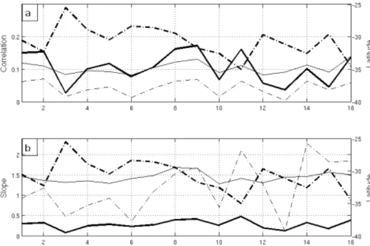
Figure 9.Correlations(a)and slopes(b)betweenT′×V′as thick continuous lines,(∇.u)′×(∂T /∂d)′ as thin continuous lines and −(∇ ×u)′×(∂T /∂c)′as thin dash-dotted lines and the mean Lat-itude (thick dash-dotted line) for the 16 Agulhas rings identified in the present study. A remarkable anti-correlation of the correlations and slopes with the latitude is observed.
negatively correlated with both the slopes and correlations (Fig. 9), while the mean wind intensity is positively corre-lated (Fig. 10). Since in this case we want to explore the in-fluence of the mean atmospheric circulation on the coupling, the mean wind is defined as the temporal mean over the ed-dies. The eddy diameters and amplitudes presented low cor-relations with the analyzed properties that are not statistically relevant.
The influence of the latitude on the coupling can be ex-plained through its impact on the thermal wind balance over the rings. A “temperature island” effect occurs due to the modifications in the heat flux over the SST anomalies. This heat flux generates pressure gradients in the lower MABL that create secondary cells of circulation. Following the ther-mal wind equation (u′g= ∇P /ρf ), the magnitude of the geostrophic wind perturbation (u′g) due to this pressure gra-dient (∇P ) is inversely proportional to the Coriolis factor (f ). Sincef is larger in higher latitudes,u′gis smaller, that is, the pressure gradient mechanism is less effective. Chel-ton et al. (2004) also observed the influence of the latitude in the air–sea coupling and affirmed that the SST influence on the mean wind stress is mostly restricted to regions pole-ward of 40◦ of latitude and the tropics, though the authors
associated this effect to the persistence of the SST fronts over time. In the present study, we show that such effects are observed in lower latitudes as well (∼30◦S) and
tran-sient fronts, which can also be interpreted from the results of O’Neill et al. (2010).
The influence of the wind velocity is associated with a dif-ferent process. It promotes modifications in the near-surface stability or, in the case of the wind curl, generates vertical velocities in the ocean that impact the SST (Ekman pump-ing). While the first case is the subject of extensive research
(e.g., Kudryavtsev et al., 1996; Park and Cornillon, 2002; Liu et al., 2007; O’Neill, 2012) and will not be treated in the present work, the second process explains an important feedback mechanism from the MABL into the ocean and is discussed in the next section.
6 Induced Eddy–Ekman pumping
As statistically revealed, wind modifications, and conse-quently wind stress, could possibly enhance vertical veloc-ities through an Ekman pumping mechanism in the ocean. This further impacts the resulting evolution of the SST field and again the surface stress. Such a coupled feedback has been less explored than the impacts of the SST gradients on the surface winds. Liu et al. (2007) discuss the feedback of the wind speed anomalies on the ocean in terms of modifica-tions in the wind stress, impacting the surface currents. The authors argue that since the neutral wind vorticity anoma-lies are small compared to those of the ocean currents, the ocean should dominate the mesoscale coupling in the long term. The feedback on the SST is then presented as function of the modifications in the surface latent heat flux. The role of the surface heat fluxes was further emphasized by Haack et al. (2008). From another point of view, using an ideal-ized ocean–atmosphere coupled model to study the shelf-break frontogenesis, Chen et al. (2003) showed a positive feedback mechanism that strengthens both the wind and the front. Their results indicate that although the latent heat flux appears to be important, it is not an essential coupling mech-anism. Jin et al. (2009) used the empirical relationship be-tween the wind and SST presented by Chelton et al. (2007), leading to a simple representation of the mesoscale ocean– atmosphere coupling in an idealized upwelling system where the SST-induced wind curl intensification strengthen the off-shore upwelling through Ekman pumping.
Under the present analysis, a more direct estimation can be made. To quantify the mean eddy–wind interactions, an f plane approximation in the eddy-centered reference frame is considered to estimate the mean Ekman vertical velocities (wEK), also taking into account the oceanic geostrophic eddy vorticity (ζ)changes obtained from the geostrophic veloci-ties derived from the observed SLA in the rings area (e.g., Stern, 1965):
wEK= 1 ρ0
∇ ×τ
f+ζ | {z }
term 1
+ ∇ζ
(f+ζ)2×τ
| {z }
term 2
, (1)
whereρ0 is the averaged oceanic mixed layer density, ob-tained considering a mean salinity of 35 and the observed SST, andτ is the wind stress simply obtained from a bulk relationship:
Figure 10.Correlations(a)and slopes(b)betweenT′×V′ (thick continuous line), (∇.u)′×(∂T /∂d)′ (thin continuous line) and −(∇ ×u)′×(∂T /∂c)′ (thin dash-dotted line) and the mean wind speed (thick dash-dotted line) for the 16 Agulhas rings identified in the present study. A remarkable concordance between the correla-tions and slopes with the wind speed is observed.
whereρAIRis the air density,CDis the drag coefficient andV is the measured surface wind. CD was calculated following Yelland and Taylor (1996). It is important to notice that for the Ekman pumping calculation the effect of the ocean cur-rents on the observed scatterometer winds was not removed since the movement in relation to the ocean surface is the relevant quantity.
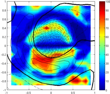
The two terms ofwEKin Eq. (1) take into account the par-ticular contribution of the resulting wind stress curl, through the measured surface wind curl anomalies (term 1), and the oceanic vorticity divergence (term 2). As presented in Fig. 11,wEKestimations overlay very well with theT′field. The high correlation (0.9) between the two fields is illus-trated in Fig. 12. The linear fit obtained between these two fields presents a−0.04 slope. In this figure it is possible to observe that this linear relationship is strong in the region close to the eddy core, weakening with the distance from it. This means that this process holds only for the region under the influence of the eddy.
As clearly revealed, the Ekman pumping explains a per-sistent feedback mechanism linking the eddy-induced mean wind and SST anomalies on the Agulhas rings. Along their propagation in the South Atlantic basin, a residual persistent upward velocity acts to support a cooler temperature flux to sustain the mean observed cool anomalies in the core of the eddies. This mechanism is mostly driven by the observed re-sulting spatial changes in wind stress, but taking into account that the oceanic vorticity gradient improves the overall cor-relation betweenwEKandT′, particularly contributing to the enhancement of the pumping asymmetry along cross-wind mean directions. As such, this observed asymmetry might lead to weaker SSH signatures, also impacting the ring prop-agation and attenuation (Dewar and Flierl, 1987). In fact, the
Figure 11.Results obtained for(a)term 1,(b)term 2 and(c)the to-tal Ekman pumping velocitywEK(m day−1)for the mean estimated Agulhas ring. A remarkable concordance is observed between the mean vertical velocities (color contours) and the observed mean T′ (black contours – c.i. 0.01◦C). ThewEK is dominated by the (∇ ×τ)′ (term1), though the(∇ ×ζ)′ (term 2) makes an impor-tant contribution. The figures’ axes represent the distances from the eddy center normalized by the eddy diameters.
relative contribution of term 2 of Eq. (1) to the total wEK displayed in Fig. 13 clearly shows that this term is responsi-ble for up to 95 % of the total vertical velocities in the lower (southern) portion of the ring. Considering the role of the mean eddy, term 2 accounts for, approximately, 30 % of the totalwEK.
Figure 12.Relationship between the Ekman pumping vertical ve-locities (wEK)andT′. The color code represent the distance from the eddy center (km), showing that the linear relationship between these two fields is stronger closer to the eddy core, as demonstrated by the linear regression illustrated by the red line.
core as described by Lehahn et al. (2011), who observed a chlorophyll patch transported by an eddy along∼1500 km in∼11 months. Based on a ring first identified in April 2006, and using a particle transport model, these authors conclude that the water trapped inside the eddy core and changes in the mixed layer depth are responsible for the observed patches. The increase in the vertical mixing by particularly strong wind events is described as responsible for high frequency increments on the chlorophyll concentration. However, the present results revealed a persistent mean mechanism, sus-taining positivewEKat the eddy cores that are consistent with the observed high productivities. As showed in Fig. 10, the mean wind speed is in fact well correlated with both the slope and correlation of the (∇ ×u)′×(∂T /∂c)′, which explains the concordance between the chlorophyll concentration and the wind speed observed by Lehahn et al. (2011).
7 Conclusions
Using three independent data sets (TMI/AMSR-E SST fields, Argo profiling floats and a blended winds product), the present study reveals a particular surface thermal signature for the anticyclonic Agulhas rings as they propagate across the South Atlantic Ocean: cold T′ in the eddy cores with warm anomalies at the boundaries. Consequently, in the in-terior of the South Atlantic basin the Agulhas rings are better described asT′dipoles, presenting strong positive and
neg-ative anomalies, than by the classical view of a warm core anticyclone that is consistent close to their formation region in the Cape Basin. These anomalies decrease in amplitude along the eddy tracks, but are still distinguishable during their whole lifetimes, estimated from the SLA.
A statistical analysis of the surface wind modifications over anticyclonic Agulhas rings is explored. The joint use of SSH, SST, and wind available products with improved
Figure 13.Relative contribution (%) of term 2 of Eq. (1) to the total Ekman pumping vertical velocity (wEK)in a mean Agulhas ring and the observed meanT′ (black contours – c.i. 0.01◦C). It is possible to ascribe the particular importance of this term to the asymmetry ofwEK andT′with higher contributions (up to 95 %) in the lower (southern) part of the eddy.
spatiotemporal resolution helps to reveal persistent effects taking place over these long-lived large mesoscale rings. Impacts of their thermal and circulation surface signatures on the wind field were ascertained in the V′, (∇.u)′ and
(∇ ×u)′wind anomaly fields. The mean spatial patterns of V′ andT′show remarkable correlation, maximum value of
0.92, with a spatial shift on the order of one quarter of the ring radius to the right of the mean wind direction. Since the Agulhas rings propagate in a region dominated by the west-erly winds, this is to say that the wind anomaly is shifted poleward (approximately 0.5◦) to the eddy thermal center.
Acknowledgements. The authors would like to thank Patrice Klein, Clement de Boyer Montegut, Cecile Cabanes and Pierre-Yves Le Traon for the fruitful discussions we had about this work. We also acknowledge the AVISO service website maintained by CLS for making publicly available their sea surface height data. Argo data were collected and made freely available by the International Argo Program and the national programs that contribute to it (http://www.argoucsd.edu, http://argo.jcommops.org). João Marcos Souza was funded through an IFREMER postdoctoral fellowship.
Edited by: S. Josey
References
Arhan, M., Speich, S., Messager, C., Dencausse, G., Fine, R., and Boye, M.: Anticyclonic and cyclonic eddies of subtropical origin in the subantarctic zone of south of Africa, J. Geophys. Res., 116, C11004, doi:10.1029/2011JC007140, 2011.
Bentamy, A., Ayina, H.-L., Queffeulou, P., Croize-Fillon, D., and Kerbaol, V.: Improved near real time surface wind resolution over the Mediterranean Sea, Ocean Sci., 3, 259–271, doi:10.5194/os-3-259-2007, 2007.
Biastoch, A., Boning, C. W., and Lutjeharms, J. R. E.: Agulhas leak-age dynamics affects decadal variability in the Atlantic overturn-ing circulation, Nature, 456, 489–492, 2008.
Businger, J. A. and Shaw, W. J.: The response of the marine at-mospheric boundary layer to mesoscale variations in sea-surface temperature, Dyn. Atmos. Oceans, 8, 267–281, 1984.
Byrne, D. A., Gordon, A. L., and Haxby, W. F.: Agulhas eddies: A synoptic view using Geosat ERM data, J. Phys. Oceanogr., 25, 902–917, 1995.
Chaigneau, A., Eldin, G., and Dewitte, B.: Eddy activity in the four major upwelling systems from satellite altimetry (1992–2007), Prog. Oceanogr., 83, 117–123, 2009.
Chelton, D. B., Esbensen, S. K., Schlax, M. G., Thum, N., Freilich, M. H., Wentz, F. J., Gentemann, C. L., McPhaden, M. J., and Schopf, P. S.: Observations of coupling between surface wind stress and sea surface temperature in the eastern tropical Pacific, J. Climate, 14, 1479–1498, 2001.
Chelton, D. B., Schlax, M. G., Freilich, M. H., and Milliff, R. F.: Satellite measurements reveal persistent small-scale features in ocean winds, Science, 303, 978–983, 2004.
Chelton, D. B., Schlax, M. G., and Samelson, R. M.: Summer-time coupling between sea surface temperature and wind stress in the California Current System, J. Phys. Oceanogr., 37, 495–517, 2007.
Chelton, D. B., Schlax, M. G., and Samelson, R. M.: Global Ob-servations of Nonlinear Mesoscale Eddies, Prog. Oceanogr., 91, 167–216, 2011.
Chen, D., Timothy, W., Tang, W., and Wang, Z.: Air-sea in-teraction at an oceanic front: Implications for frontogene-sis and primary production. Geophys. Res. Lett., 30, 1745, doi:10.1029/2003GL017536, 2003.
Dencausse, G., Arhan, M., and Speich, S.: Routes of Agulhas rings in the southeastern Cape Basin, Deep-Sea Res I, 57, 1406–1421, 2010.
Dewar, W. K. and Flierl, G. R.: Some effects of the wind on rings, J. Phys. Oceanogr., 17, 1653–1667, 2007.
Flierl, G. R.: Particle motions in large-amplitude wave fields, Geo-phys. Astro. Fluid, 18, 39–74, 1981.
Frenger, I., Gruber, N., Knutti, R., and Münnich, M.: Imprint of Southern Ocean eddies on winds, clouds and rainfall, Nat. Geosci., 6, 608–612, doi:10.1038/NGEO1863, 2013.
Garzoli, S. L., Richardson, P. L., Duncombe Rae, C. M., Fratantoni, D. M., Goni, G. J., and Roubicek, A. J.: Three Agulhas rings observed during the Benguela Current Experiment, J. Geophys. Res., 104, 20971–20985, 1999.
Gladyshev, S., Arhan, M., Sokov, A., and Speich, S.: A hydro-graphic section from South Africa to the southern limit of the Antarctic Circumpolar Current at the Greenwich meridian, Deep-Sea Res. I, 55, 1284–1303, 2008.
Haack, T., Chelton, S. D., Pullen, J., Doyle, J., and Schlax, M.: Air-sea interaction from U. S. West Coast summertime forecasts. J. Phys. Oceanogr., 38, 2414–2437, 2008.
Jin, X., Dong, C., Kurian, J., and McWilliams, J.: SST-Wind interaction in coastal upwelling: Oceanic simulation with empirical coupling, J. Phys. Oceanogr., 39, 2957–2970, doi:10.1175/2009JPO4205.1, 2009.
Kudryavtsev, V. N., Grodsky, S. A., Dulov, V. A., and Malinovsky, V. V.: Observations of atmospheric boundary layer evolution above the Gulf Stream frontal zone, Bound-Lay. Meteorol., 79, 51–82, 1996.
Kudryavtsev, V. N., Akimov, D., Johannessen, J., and Chapron, B.: On radar imaging of current features: 1. Model and com-parison with observations, J. Geophys. Res., 110, C07016, doi:10.1029/2004JC002505, 2005.
Lehahn, Y., d’Ovidio, F., Lévy, M., Amitai, Y., and Heifetz, E.: Long range transport of a quasi isolated clorophyll patch by an Agulhas ring, Geophys. Res. Lett., 38, L16610, doi:10.1029/2011GL048588, 2011.
Liu, W. T., Xie, X., and Niiler, P.: Ocean-atmosphere interaction over Ahulhas Extension meanders, J. Climate, 20, 5784–5797, 2007.
O’Neill, L. W.: Wind speed and stability effects on the coupling between surface wind stress and SST observed from buoys and satellite, J. Climate, 25, 1544–1569, doi:10.1175/JCLI-D-11-00121.1, 2012.
O’Neill, L. W., Chelton, D. B., and Esbensen, S. K.: High-Resolution Satellite Measurements of the Atmospheric Bound-ary Layer response to SST Variations along the Agulhas Return Current, J. Climate, 18, 2706–2723, 2005.
O’Neill, L. W., Chelton, D. B., and Esbensen, S. K.: The effects of SST-induced surface wind speed and direction gradients on midlatitude surface vorticity and divergence, J. Climate, 23, 255– 281, 2010.
Park, K. and Cornillon, P. C.: Stability-induced modification of sea surface winds over Gulf Stream rings, Geophys. Res. Lett., 29, 2211, doi:10.1029/2001GL014236, 2002.
Park, K.-A., Cornillon, P., and Codiga, D. L.: Modification of sur-face winds near ocean fronts: Effects of Gulf Stream rings on scatterometer (QuikSCAT, NSCAT) wind observations. J. Geo-phys. Res., 111, C03021, doi:10.1029/2005JC003016, 2006. Schmid, C., Boebel, O., Zenk, W., Lutjeharms, J. R. E., Garzoli,
S. L., Richardson, P. L., and Barrong, C.: Early evolution of an Agulhas Ring, Deep-Sea Res. II, 50, 141–166, 2003.
eddies in the Sargasso Sea, Geophys. Res. Lett., 38, L13608, doi:10.1029/2011GL047660, 2011.
Small, R. J., deSzoeke, S. P., Xie, S. P., O’Neill, L., Seo, H., Song, Q., Cornillon, P., Spall, M., and Minobe, S.: Air-sea interaction over ocean fronts and eddies, Dyn. Atmos. Oceans, 45, 274–319, 2008.
Souza, J. M. A. C., de Boyer Montégut, C., and Le Traon, P. Y.: Comparison between three implementations of automatic iden-tification algorithms for the quaniden-tification and characterization of mesoscale eddies in the South Atlantic Ocean, Ocean Sci., 7, 317–334, doi:10.5194/os-7-317-2011, 2011a.
Souza, J. M. A. C., de Boyer Montégut, C., Cabanes, C., and Klein, P.: Estimation of the Agulhas ring impacts on meridional heat fluxes and transport using ARGO floats and satellite data, Geophys. Res. Lett., 38, L21602, doi:10.1029/2011GL049359, 2011b.
Stern, M. E.: Interaction of a uniform wind stress with a geostrophic vortex, Deep-Sea Res., 12, 355–367, 1965.
van Aken, H. M., van Veldhoven, A. K., Veth, C., de Ruijter, W. P. M., van Leeuwen, P. J., Drijfhout, S. S., Whittle, C. P., and Rouault, M.: Observations of a young Agulhas Ring, Astrid, dur-ing MARE in March 2000. Deep-Sea Res. II, 50, 167–195, 2003. van Sebille, E., van Leeuwen, P. J., Biastoch, A., and Ruijter, W. P. M.: On the fast decay of Agulhas rings. J. Geophys. Res., 115, C03010, doi:10.1029/2009JC005585, 2010.